- Physical Chemistry
- Chemical Equilibria: Multiple Component Systems
Micro-courses:12

Chemical Equilibria: Multiple Component Systems
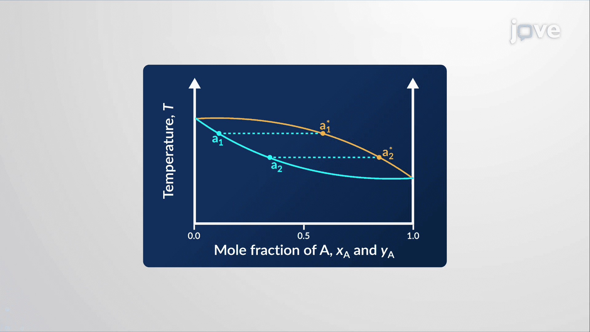
1. Two Components: Liquid–Liquid Systems
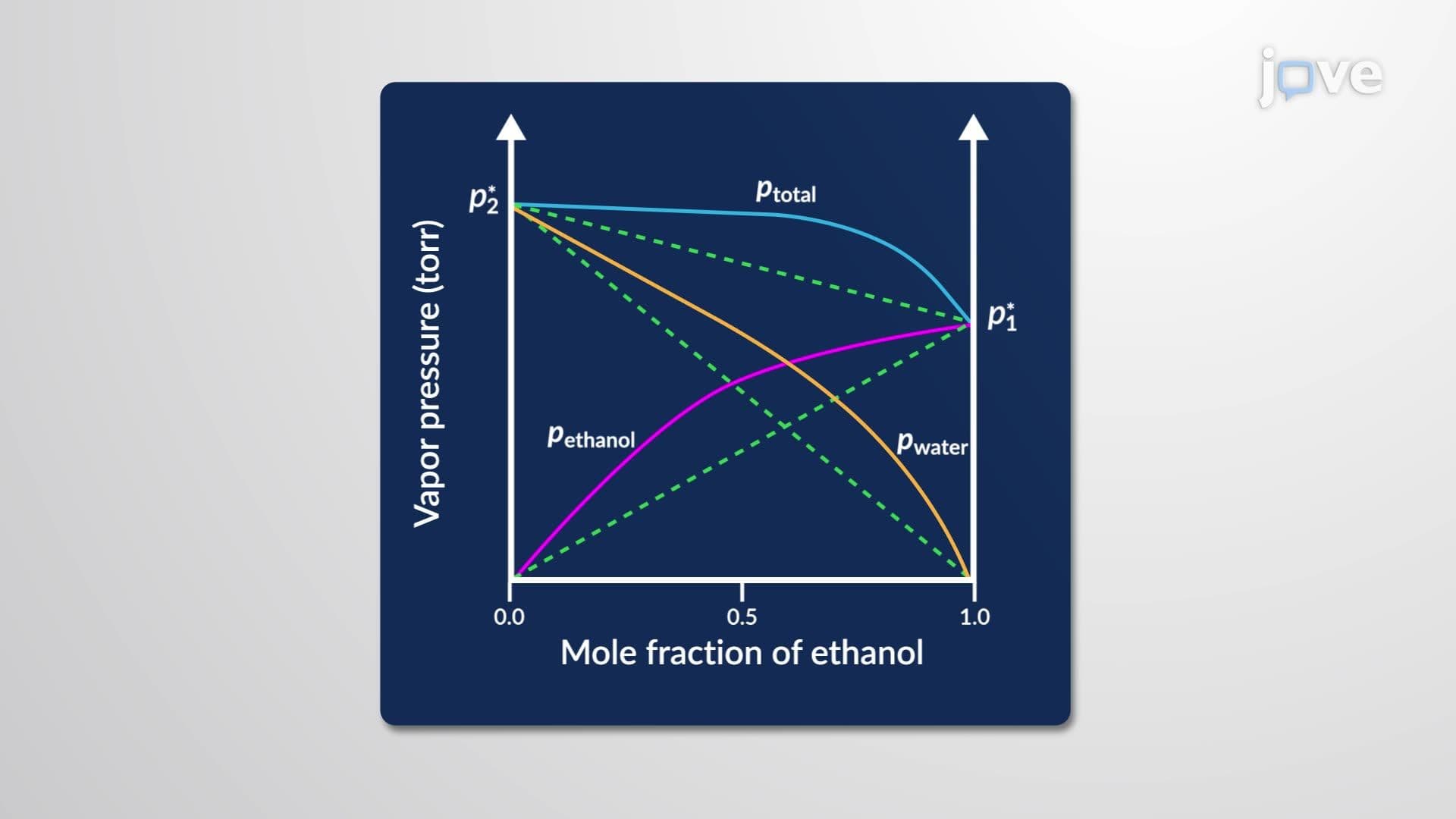
2. Nonideal Two-Component Liquid Solutions
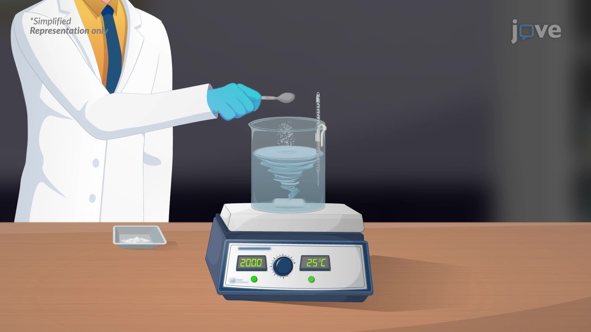
3. Liquid–Solid Solutions
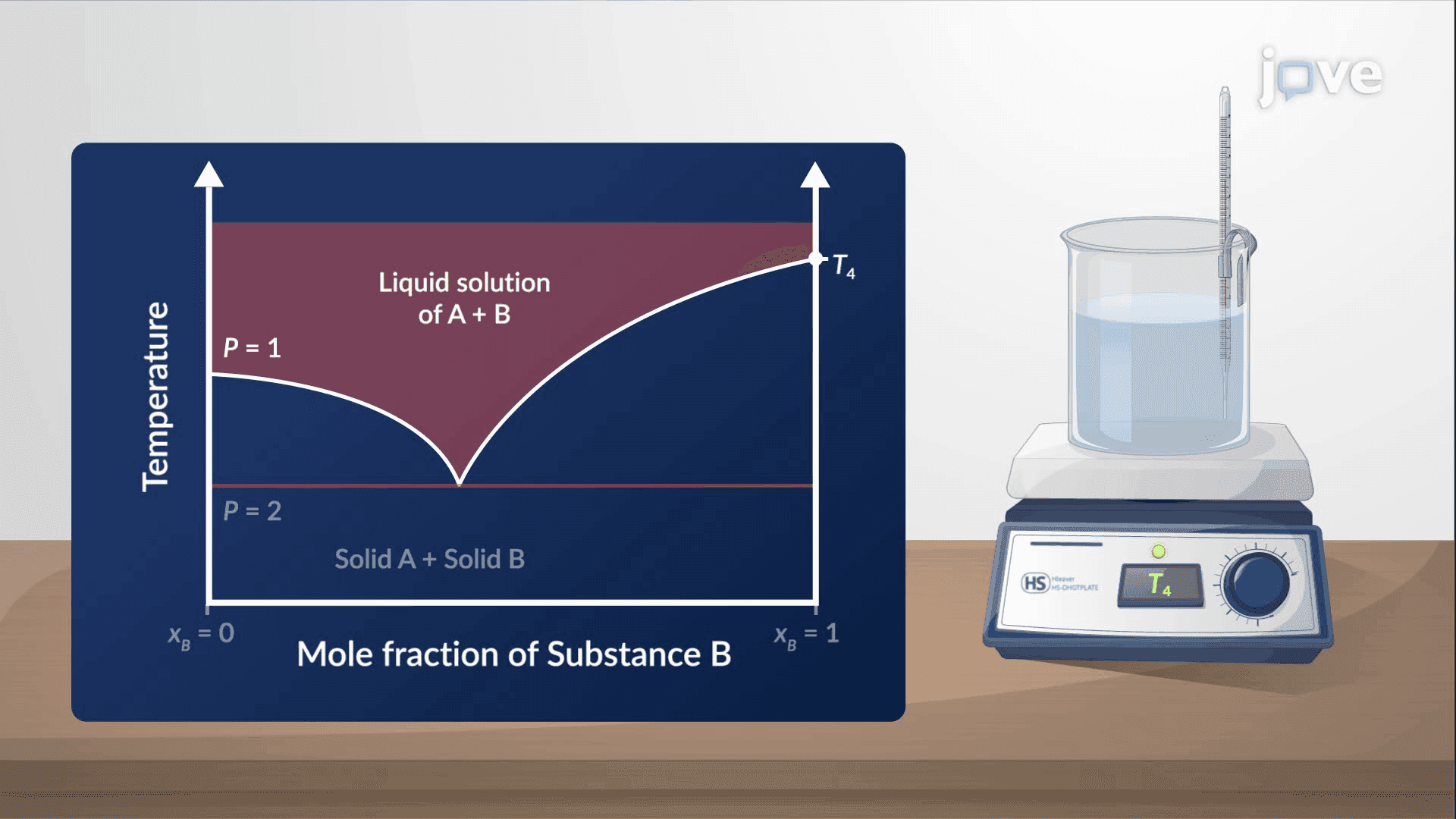
4. Solid–Solid Solutions
5. Colligative Properties
6. Freezing Point Depression and Boiling Point Elevation
7. Osmotic Pressure
8. Phase Diagrams of Ternary Systems
Chemical Equilibria in multiple component systems governs everything from industrial distillation towers in Texas refineries to IV fluid formulation in US hospitals. This micro-course, supported by JoVE Coach, explores how two- and three-component mixtures behave across liquid-liquid, liquid-solid, and solid-solid phases. Students examine phase diagrams, azeotropes, eutectic mixtures, colligative properties, osmotic pressure, and ternary systems using thermodynamic principles grounded in real-world chemistry.
- Understand how pressure-composition and temperature-composition phase diagrams describe equilibrium behavior in two-component liquid systems
- Identify ideal versus nonideal solution behavior and explain deviations from Raoult's law using molecular interaction principles
- Analyze azeotropic compositions and explain why minimum- and maximum-boiling azeotropes resist separation by standard fractional distillation
- Explore solid solubility in liquid-solid solutions through thermodynamic parameters including Gibbs energy of fusion, enthalpy, and entropy
- Apply the eutectic concept to solid-solid phase diagrams, identifying eutectic composition, eutectic halt, and two-phase regions
- Understand how colligative properties — vapor pressure lowering, freezing point depression, boiling point elevation, and osmotic pressure — depend on solute concentration rather than solute identity
- Learn how the van't Hoff equation and expanded osmotic virial coefficient equation determine molar masses of polymers and macromolecules
- Analyze ternary phase diagrams using triangular coordinates, identifying the binodal curve, tie lines, and the plait point
1. Pressure-Composition and Temperature-Composition Phase Diagrams for Ideal Binary Liquid Systems
For an ideal two-component liquid solution — such as benzene and toluene — the pressure-composition phase diagram displays a bubble point line (liquid mole fraction vs. pressure) and a dew point line (vapor mole fraction vs. pressure). A horizontal tie line connects coexisting liquid and vapor compositions at any given equilibrium pressure. Temperature-composition diagrams work analogously: the liquid line marks boiling temperatures across compositions, and the vapor line tracks equilibrium vapor compositions. An isopleth — a vertical constant-composition line — shows how a system moves through phases as temperature or pressure changes. These diagrams form the foundation for understanding fractional distillation design in US petrochemical refineries.
2. Nonideal Solutions and Azeotropes
Real solutions deviate from Raoult's law when solute-solvent molecular interactions differ from solute-solute and solvent-solvent interactions. Strong solute-solvent attraction — as in acetone-chloroform mixtures — reduces vapor pressure below ideal predictions, producing a negative deviation. Weak cross-interactions — as in ethanol-water mixtures — raise vapor pressure above ideal predictions, producing a positive deviation. On a temperature-composition diagram, these deviations create an azeotrope: a specific composition where bubble and dew point lines intersect. At this point, liquid and vapor phases share identical compositions, so standard distillation cannot separate them further. Positive-deviation systems form minimum-boiling azeotropes; negative-deviation systems form maximum-boiling azeotropes. The ethanol-water azeotrope (95.6% ethanol) is a classic US industrial example encountered in fuel-grade ethanol production.
3. Liquid-Solid Solutions and Solubility
When a solid dissolves in a liquid, dissolution continues until the solution reaches its solubility limit, at which point the solution is saturated and the chemical potential of dissolved and undissolved solute are equal. For an ideal liquid-solid solution, solubility can be expressed mathematically using the solute's mole fraction, which depends on the Gibbs energy of fusion, enthalpy of fusion, entropy of fusion, and the solute's melting point. This framework reveals a key principle: solutes with higher melting points tend to be less soluble at a given temperature. This thermodynamic approach explains, for example, why aspirin (a high-melting-point compound) has limited solubility in water at room temperature — a consideration critical to US pharmaceutical formulation.
4. Solid-Solid Solutions and Eutectic Systems
When two mutually insoluble solids — such as bismuth and cadmium, studied historically in US metallurgy — form completely miscible liquids, their temperature-composition phase diagram reveals a characteristic eutectic point. Cooling a liquid mixture causes one pure solid component to crystallize first, enriching the remaining liquid in the other component. This continues until the liquid reaches the eutectic composition, the mixture with the absolute lowest melting point. At this composition, the system freezes at a single, constant temperature — a phenomenon called the eutectic halt — producing a two-phase solid of pure A and pure B. Eutectic behavior is critical in solder alloy design and in understanding igneous rock solidification studied in US geology and materials engineering programs.
5. Colligative Properties and Vapor Pressure Lowering
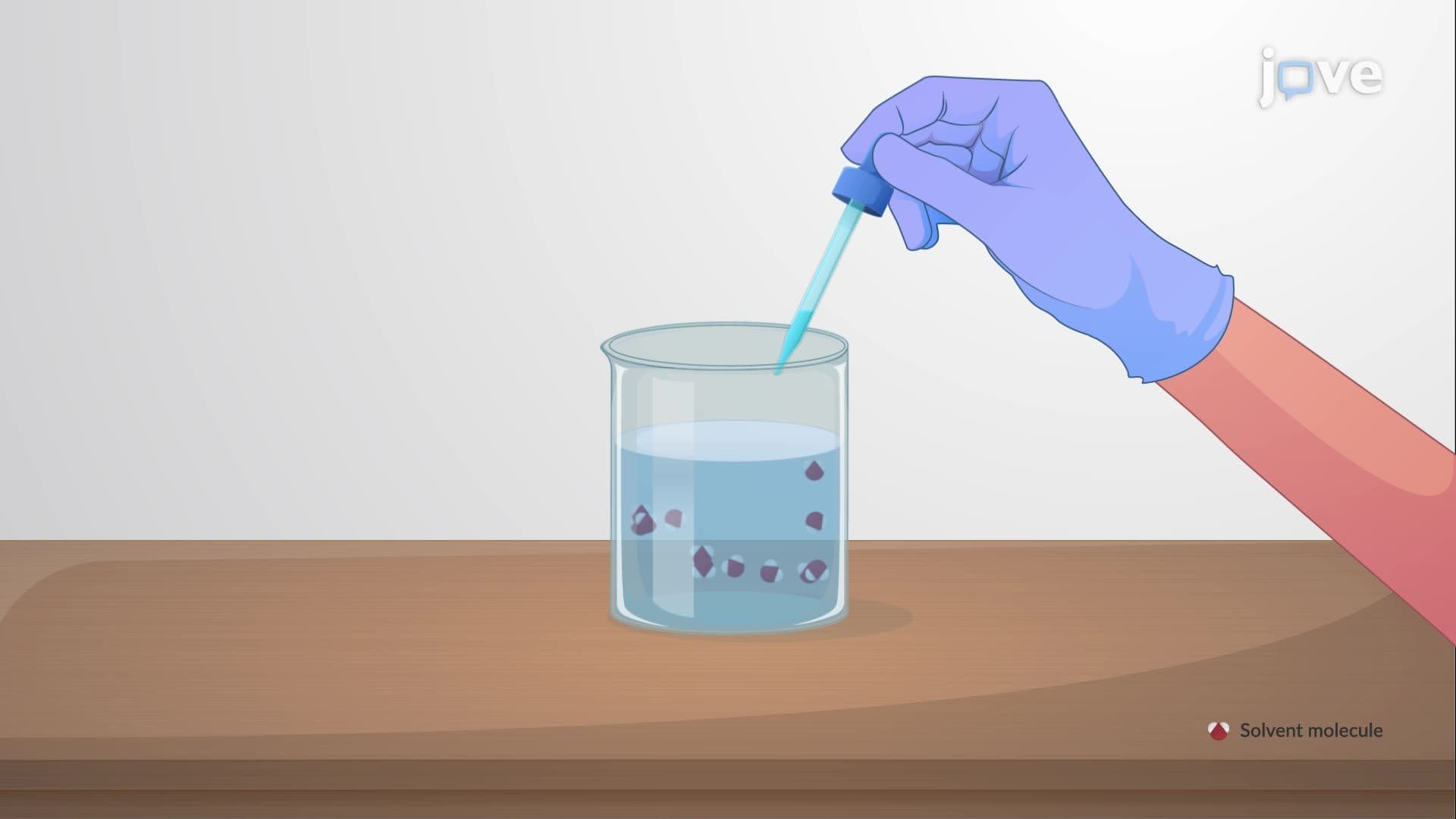
Colligative properties depend solely on the number of dissolved solute particles, not their chemical identity. When a nonvolatile solute is added to a pure solvent, it reduces the solvent's mole fraction and therefore lowers the solvent's chemical potential. This reduction directly decreases the solution's equilibrium vapor pressure relative to the pure solvent — a relationship described by Raoult's law for dilute ideal solutions. The change in vapor pressure equals the product of the solute's mole fraction and the pure solvent's vapor pressure. This principle is applied in US industries ranging from antifreeze formulation (ethylene glycol in coolants) to food preservation, where dissolved sugars and salts lower the water activity of products.
6. Freezing Point Depression and Boiling Point Elevation
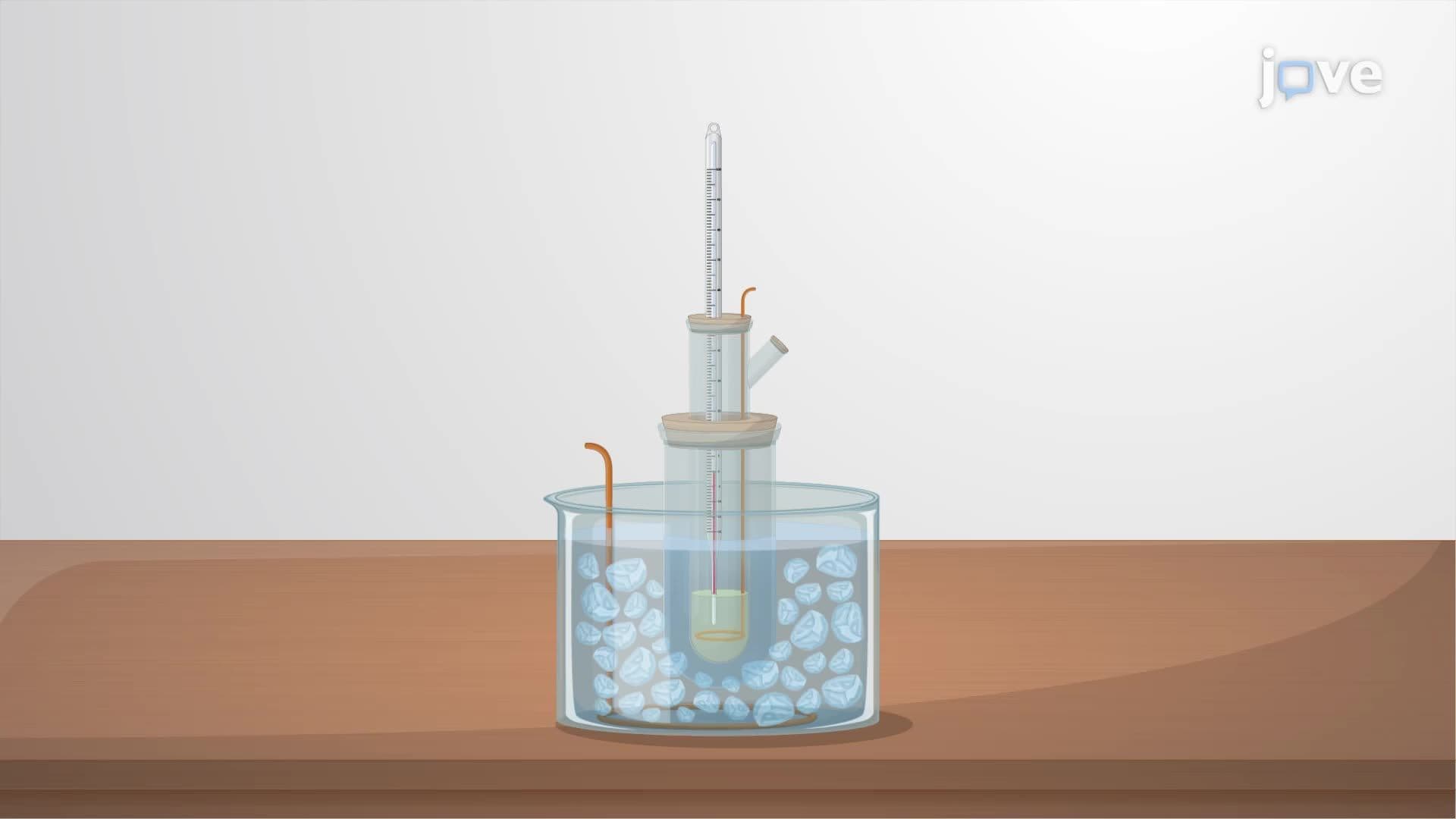
Adding a nonvolatile solute to a solvent shifts the chemical potential of the liquid phase downward without affecting the solid or vapor phases. On a chemical potential versus temperature plot, this shift moves the liquid-solid intersection to a lower temperature (freezing point depression) and the liquid-vapor intersection to a higher temperature (boiling point elevation). Quantitatively, freezing point depression equals the product of the solute's molality and the solvent's cryoscopic constant (Kf); boiling point elevation equals molality times the ebullioscopic constant (Kb). These effects explain why road salt lowers the freezing point of water on US highways in winter, and why dissolved solutes raise pasta-water's boiling point — though the latter effect is negligible at culinary concentrations.
7. Osmotic Pressure
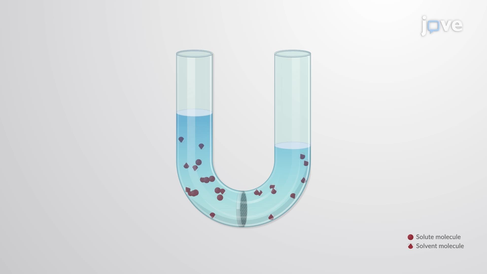
Osmosis is the net movement of solvent molecules through a semipermeable membrane from a region of lower solute concentration to higher solute concentration. The pressure required to stop this flow is the osmotic pressure (π), calculated for ideal dilute solutions using the van't Hoff equation: π = MRT, where M is molar concentration, R is the gas constant, and T is absolute temperature. For nonideal solutions of macromolecules — such as proteins or synthetic polymers studied in US biomedical research — an expanded van't Hoff equation incorporating the osmotic virial coefficient (B) corrects for excluded volume and intermolecular interactions. Plotting π/c_mass vs. c_mass allows researchers to determine polymer molar mass from the y-intercept and the virial coefficient from the slope — a technique used in US polymer laboratories for quality control.
8. Phase Diagrams of Ternary Systems
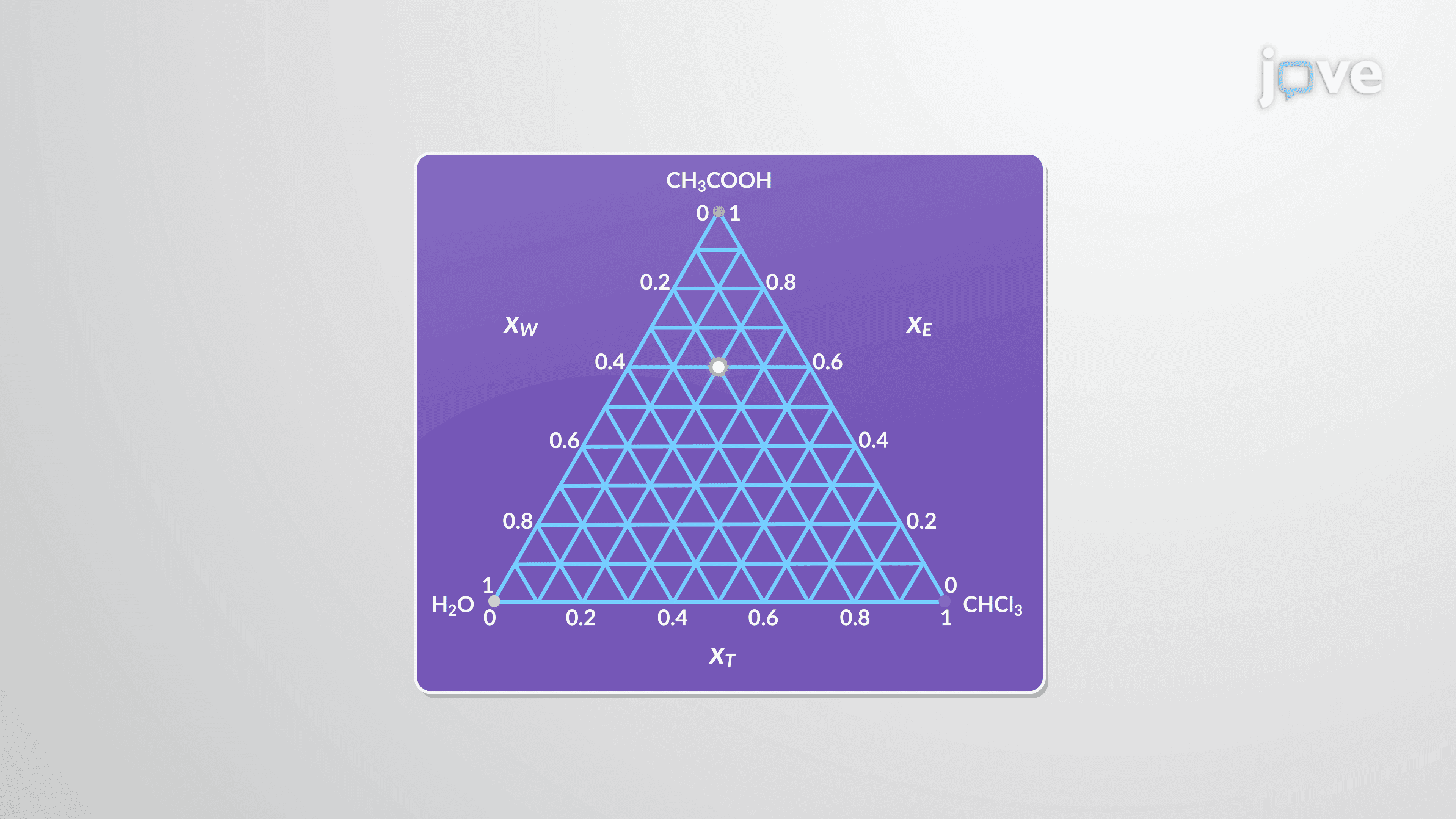
A ternary phase diagram represents three-component systems on an equilateral triangle, where each vertex is a pure component, each edge is a binary mixture, and interior points represent all three components present simultaneously. The binodal curve encloses the two-phase region. A classic example is the water–trichloromethane–ethanoic acid system: water and trichloromethane are only partially miscible, but ethanoic acid (acetic acid) is fully miscible with both. Adding acetic acid increases mutual solubility of water and trichloromethane, shrinking the two-phase region. The plait point marks where the two liquid phases become compositionally identical and merge into one. Ternary diagrams guide liquid-liquid extraction processes used in US pharmaceutical and chemical manufacturing to optimize solvent selection.
Frequently Asked Questions
The bubble point line marks the pressure (or temperature) at which a liquid mixture just begins to vaporize — the first bubble of vapor appears. The dew point line marks the condition at which a vapor mixture just begins to condense — the first drop of liquid forms. In a pressure-composition diagram, the bubble point line lies above the dew point line. The region between the two lines is a two-phase zone where both liquid and vapor coexist, connected at any given pressure by a horizontal tie line. ---
At the azeotropic composition, the liquid and vapor phases have exactly the same mole fractions. Because distillation separates components by exploiting differences in vapor and liquid compositions, and because no such difference exists at the azeotrope, the mixture distills as if it were a single pure substance — boiling at a constant temperature without changing composition. This is why the ethanol-water azeotrope (≈95.6% ethanol by mass) cannot be concentrated further by simple distillation. US fuel-ethanol producers use molecular sieves or azeotropic distillation with a third component (entrainer) to break this limitation and reach anhydrous ethanol. ---
On the AP Chemistry exam, colligative properties — especially freezing point depression and osmotic pressure — are frequently tested in free-response questions involving molality calculations, van't Hoff factors for electrolytes, and comparing solution behaviors. On the MCAT, osmotic pressure is especially important in the context of biological membranes, IV solution tonicity (isotonic vs. hypertonic vs. hypotonic), and kidney function. You should be comfortable calculating ΔTf = Kf × m and π = MRT, and understanding that electrolytes like NaCl contribute more particles per formula unit, amplifying colligative effects. ---
Both. AP Chemistry covers colligative properties (freezing point depression, boiling point elevation, osmotic pressure, vapor pressure lowering) and basic phase diagram interpretation. However, topics like nonideal solutions, azeotropes, eutectic phase diagrams, osmotic virial coefficients, and ternary systems are standard in college-level general chemistry and physical chemistry courses. Students in university programs — particularly those studying chemistry, chemical engineering, or biochemistry — will encounter the full depth of this material in courses aligned with ACS curriculum guidelines. ---
Eutectic systems are widely applied in US industry. Lead-tin solders historically used in electronics exploit eutectic compositions to achieve sharp melting points for clean, reliable joints. Road deicers — including salt-sand mixtures and magnesium chloride blends used by US state departments of transportation — leverage freezing point depression related to eutectic behavior. In US geology, eutectic points explain how igneous rocks crystallize from magma; mineralogists study binary and ternary eutectic diagrams to model mineral formation in cooling magma chambers. Even ice cream production uses eutectic salt-ice mixtures to achieve temperatures below 0°C during hand-cranked churning. ---
Most students find nonideal solution behavior and azeotropes challenging because it requires connecting molecular-level interactions to macroscopic phase diagram features — and then applying that understanding to a practical distillation scenario. A strong approach is to work in three steps: (1) First, master ideal solutions and Raoult's law as your baseline. (2) Then, ask whether intermolecular forces between unlike molecules are stronger or weaker than those between like molecules — this determines the direction of deviation. (3) Finally, sketch the temperature-composition diagram and locate the azeotrope visually before attempting any calculations. Pairing diagram interpretation with worked problems dramatically improves retention. ---
The lever rule is a mass-balance tool used in two-phase regions of a phase diagram to determine the relative amounts (not just compositions) of each phase present at equilibrium. Once you draw a tie line at a given temperature or pressure connecting the two coexisting phase compositions, the lever rule states that the fraction of one phase equals the length of the tie line segment on the opposite side divided by the total tie line length. For example, in a binary liquid-vapor system, if your overall composition sits closer to the liquid end of the tie line, most of the system is liquid — a small amount is vapor. This quantitative insight is essential in industrial flash calculations used in US refinery distillation column design. ---
Start by memorizing the vocabulary (tie line, isopleth, bubble point, dew point, eutectic, plait point, binodal curve) before attempting to interpret specific diagrams — you cannot read a map without knowing what the symbols mean. Next, practice tracing system paths: pick a point on a diagram and describe what happens as temperature or pressure changes step by step. Use US textbook resources such as Atkins' Physical Chemistry or Levine's Physical Chemistry for practice problems. For ternary diagrams specifically, practice plotting compositions on triangular graph paper until locating interior points becomes intuitive. Finally, connect each diagram type to a concrete application — this anchors abstract concepts in memory and is especially useful for open-ended exam questions.
This microcourse includes 8 concept videos that walk you through the building blocks of Physical Chemistry. Each video is short, about 1 minute, so you can cover a full topic during a coffee break or between classes. The full sequence starts with Two Components: Liquid–Liquid Systems and ends with Phase Diagrams of Ternary Systems.
The playlist moves from big-picture ideas to the precise vocabulary used in Physical Chemistry. Early videos introduce Two Components: Liquid–Liquid Systems, Nonideal Two-Component Liquid Solutions, and Liquid–Solid Solutions. The middle of the series focuses on Colligative Properties, Freezing Point Depression and Boiling Point Elevation, and Osmotic Pressure. The final stretch covers Phase Diagrams of Ternary Systems.
The natural next step is Nonideal Solutions. From there, you can move to Electrochemistry I: Electrolytic Conductance and Transference, Electrochemistry II: Electrochemical Systems, and Chemical Kinetics. Once you finish those, the full Physical Chemistry curriculum of 12 microcourses on JoVE Coach opens up, taking you from foundational concepts to advanced systems.
Related Subjects