Transmission-Line Differential Equations

• Understand What are Transmission Line Differential Equations and how they describe voltage and current relationships in electrical transmission systems
• Identify the key components of transmission line models including series impedance and shunt admittance per unit length
• Analyze how Kirchhoff's laws lead to second-order differential equations governing transmission line behavior
• Apply the concept of lossless lines to simplify complex transmission line calculations
• Recognize the significance of propagation constants and characteristic impedance in transmission line analysis
• Evaluate ABCD parameters and their role in determining voltage and current at any point along a transmission line
• Compare short, medium, and long transmission line approximation methods used in engineering practice
• Explore the mathematical relationship between hyperbolic functions and transmission line solutions

Understanding Transmission Line Differential Equations

Lossless lines form the cornerstone of transmission line theory, representing idealized electrical pathways where energy propagates without resistive losses. These mathematical models help engineers design everything from smartphone antennas to cross-country power transmission networks that carry electricity from hydroelectric dams in the Pacific Northwest to cities across America.

Mathematical Foundation and Kirchhoff's Laws

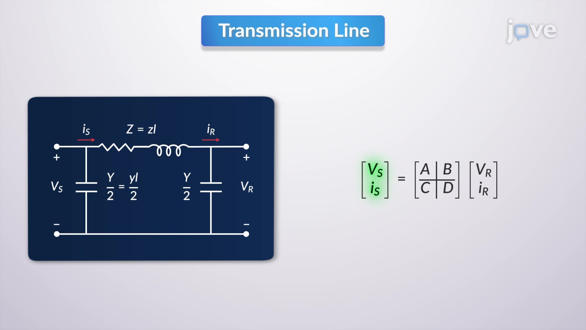
The derivation begins with a fundamental circuit model representing a small line section. Engineers define two critical parameters: series impedance (Z) and shunt admittance (Y) per unit length. By applying Kirchhoff's voltage and current laws to this infinitesimal section and taking the limit as the section length approaches zero, we obtain two coupled first-order differential equations.

When we differentiate the voltage equation and substitute it into the current equation, a second-order homogeneous differential equation emerges. This mathematical transformation reveals the wave nature of electrical signals-the same principle that allows your cell phone to communicate with towers miles away. Students preparing for the AP Physics exam or college-level electrical engineering courses will encounter similar wave equations in various contexts.

Propagation Constants and Characteristic Impedance

The solution to these differential equations involves two integration constants and introduces the propagation constant (γ), a complex quantity that determines how signals attenuate and phase-shift as they travel. For lossless lines, this constant becomes purely imaginary, indicating no amplitude decay-only phase changes occur.

The characteristic impedance (Z₀) emerges naturally from this analysis, representing the ratio of voltage to current for waves traveling in one direction. This concept proves crucial for impedance matching in RF systems, ensuring maximum power transfer in applications from radio broadcasting to satellite communications.

ABCD Parameters and Practical Applications

The final mathematical framework yields ABCD parameters-a matrix representation that relates sending-end and receiving-end voltages and currents. Electrical engineers at utilities like Pacific Gas & Electric use these parameters daily to analyze power flow and voltage regulation across transmission networks spanning hundreds of miles.

For students tackling homework problems or preparing for engineering licensing exams, understanding that these parameters apply to any line length provides computational flexibility. Short and medium-length line approximations simplify hand calculations while maintaining engineering accuracy for most practical applications.