Loading subject page…


5,235 views
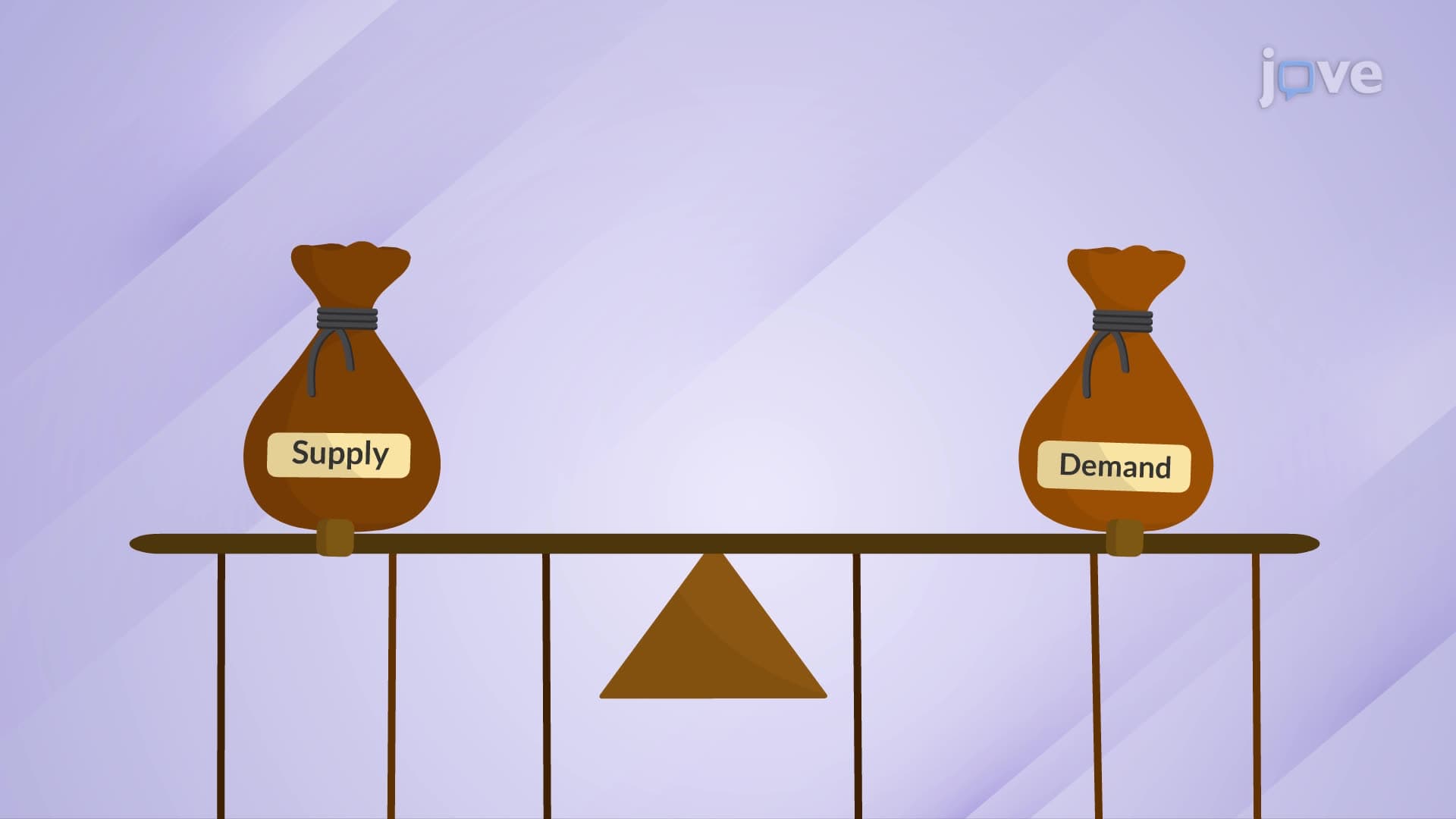

Video Summary: What Is the Mathematics of Equilibrium
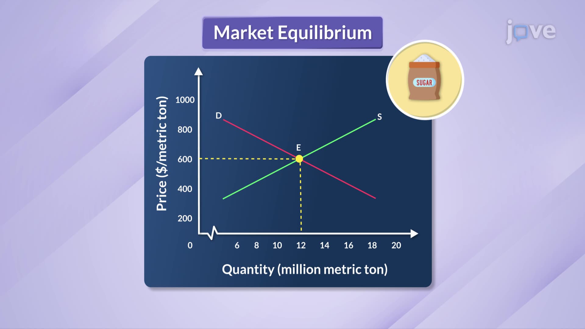
Ever wonder why a gallon of milk costs roughly the same at grocery stores across your city? The mathematics of equilibrium explains this phenomenon through precise equations that determine where supply meets demand. Using linear equations for quantity demanded and supplied, we can calculate exact equilibrium prices-like finding that sugar reaches perfect market balance at $600 per metric ton and 12 million metric tons traded. Watch the full video on JoVE Coach to master this concept with expert-led visuals and step-by-step explanations.
The mathematics of equilibrium forms the foundation of microeconomic analysis, providing precise tools to predict where markets naturally settle. Unlike descriptive economic theories, mathematical equilibrium uses algebraic equations to calculate exact prices and quantities where supply equals demand. This quantitative approach transforms abstract market forces into concrete, solvable problems that appear frequently on AP Economics exams and college microeconomics courses.
Mathematical equilibrium begins with linear equations representing market behavior. The demand equation typically takes the form Qd = a - bP, where Qd represents quantity demanded, P represents price, and the coefficients reflect consumer responsiveness to price changes. The supply equation follows Qs = c + dP format, with Qs representing quantity supplied and coefficients showing producer price sensitivity.
For example, consider the U.S. corn market. A demand equation might read Qd = 100 - 2P (millions of bushels), indicating that for every dollar increase in price per bushel, quantity demanded decreases by 2 million bushels. The corresponding supply equation Qs = 20 + 3P shows suppliers increase production by 3 million bushels for each dollar price increase.
The mathematical equilibrium occurs where Qd = Qs, creating a solvable equation. Setting 100 - 2P = 20 + 3P and solving algebraically yields P = $16 per bushel as the equilibrium price. Substituting this back into either equation gives the equilibrium quantity of 68 million bushels. This mathematical precision helps economists predict market outcomes and appears in standardized tests like the SAT Subject Test in Mathematics Level 2.
While mathematical models provide valuable insights, they rely on ceteris paribus assumptions-all other factors remaining constant. In reality, factors like weather affecting agricultural supply, consumer income changes influencing demand, or government regulations can shift these equations. The 2008 financial crisis demonstrated how mathematical equilibrium models, while useful for understanding basic market mechanics, require constant adjustment for changing economic conditions.
Understanding these mathematical tools prepares students for advanced economics coursework and professional applications in finance, policy analysis, and business strategy development.
Related Micro-courses