Loading concepts…


10 Concepts
21 Concepts
12 Concepts
8 Concepts
22 Concepts
20 Concepts
14 Concepts
12 Concepts
11 Concepts
7 Concepts
14 Concepts
8 Concepts
11 Concepts
22 Concepts
21 Concepts
21 Concepts
15 Concepts
22 Concepts
9 Concepts
6 Concepts
 20 Concepts
 6.7K Views
 Popular topics







Producer behavior examines how firms make production decisions to maximize efficiency and minimize costs. This comprehensive analysis covers fundamental principles from production functions and marginal products to advanced concepts like isoquants and returns to scale. Through real-world examples from US manufacturing, agriculture, and service industries, students explore how companies like Tesla adjust labor and capital inputs, how bakeries optimize worker allocation, and how technology transforms production processes. Master these economic principles essential for understanding modern business operations with JoVE Coach.
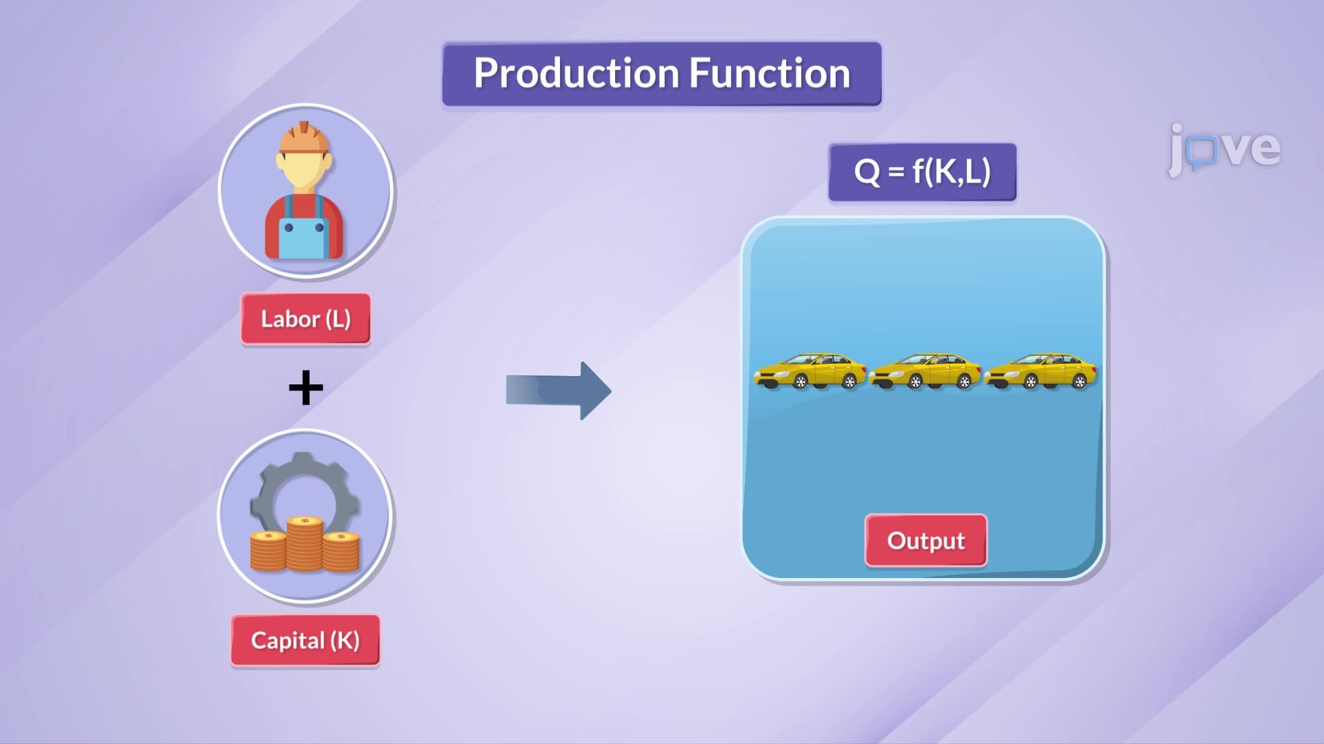
1. Production Function Fundamentals Production functions mathematically represent the relationship between inputs (labor and capital) and maximum possible output given current technology. Consider Boeing's aircraft manufacturing, where the number of planes produced depends on skilled engineers (labor) and assembly equipment (capital). The function Q = f(L,K) shows how different combinations of workers and machinery determine production capacity. Understanding this relationship helps firms like Ford Motor Company optimize their assembly lines by determining the most efficient worker-to-equipment ratios for various production targets.
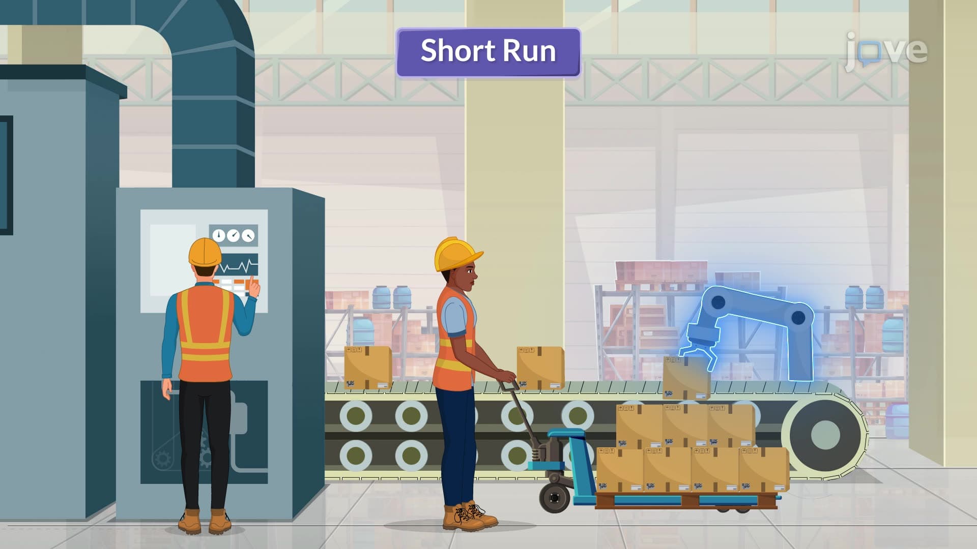
2. Short-Run vs. Long-Run Production Analysis The short-run represents periods where at least one input remains fixed, typically capital like machinery or facilities, while labor can be adjusted. McDonald's can hire more workers during busy periods but cannot immediately add new kitchen equipment. Conversely, the long-run allows firms to adjust all inputs, enabling Amazon to build new warehouses and hire additional workers simultaneously. This distinction helps businesses understand their operational flexibility and plan appropriate responses to demand changes across different time horizons.
3. Marginal Product and Diminishing Returns Marginal product measures additional output from one extra unit of input while holding others constant. In a Starbucks location with fixed espresso machines, adding the first barista significantly increases daily coffee production. However, adding a fifth barista may contribute less additional output due to equipment constraints and workspace crowding. This law of diminishing marginal returns explains why productivity eventually decreases, helping managers like those at Target determine optimal staffing levels for different store sizes and layouts.
4. Total, Average, and Marginal Product Relationships These three measures interconnect to reveal production efficiency patterns. At a clothing manufacturing plant, total product represents all garments produced daily, average product shows output per worker, and marginal product indicates additional units from hiring one more employee. When marginal product exceeds average product, the average rises; when marginal product falls below average, the average declines. Companies like Levi Strauss use these relationships to identify optimal production stages and avoid inefficient overstaffing that reduces per-worker productivity.
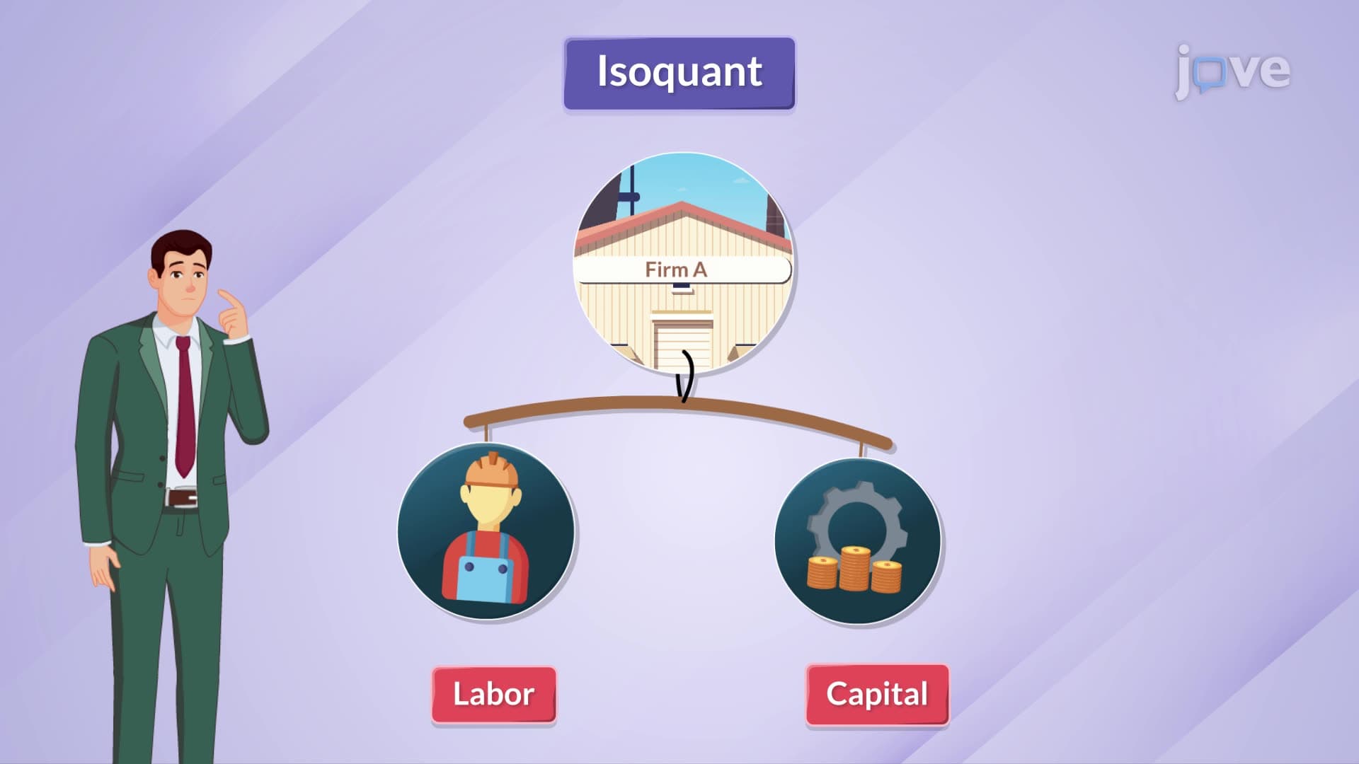
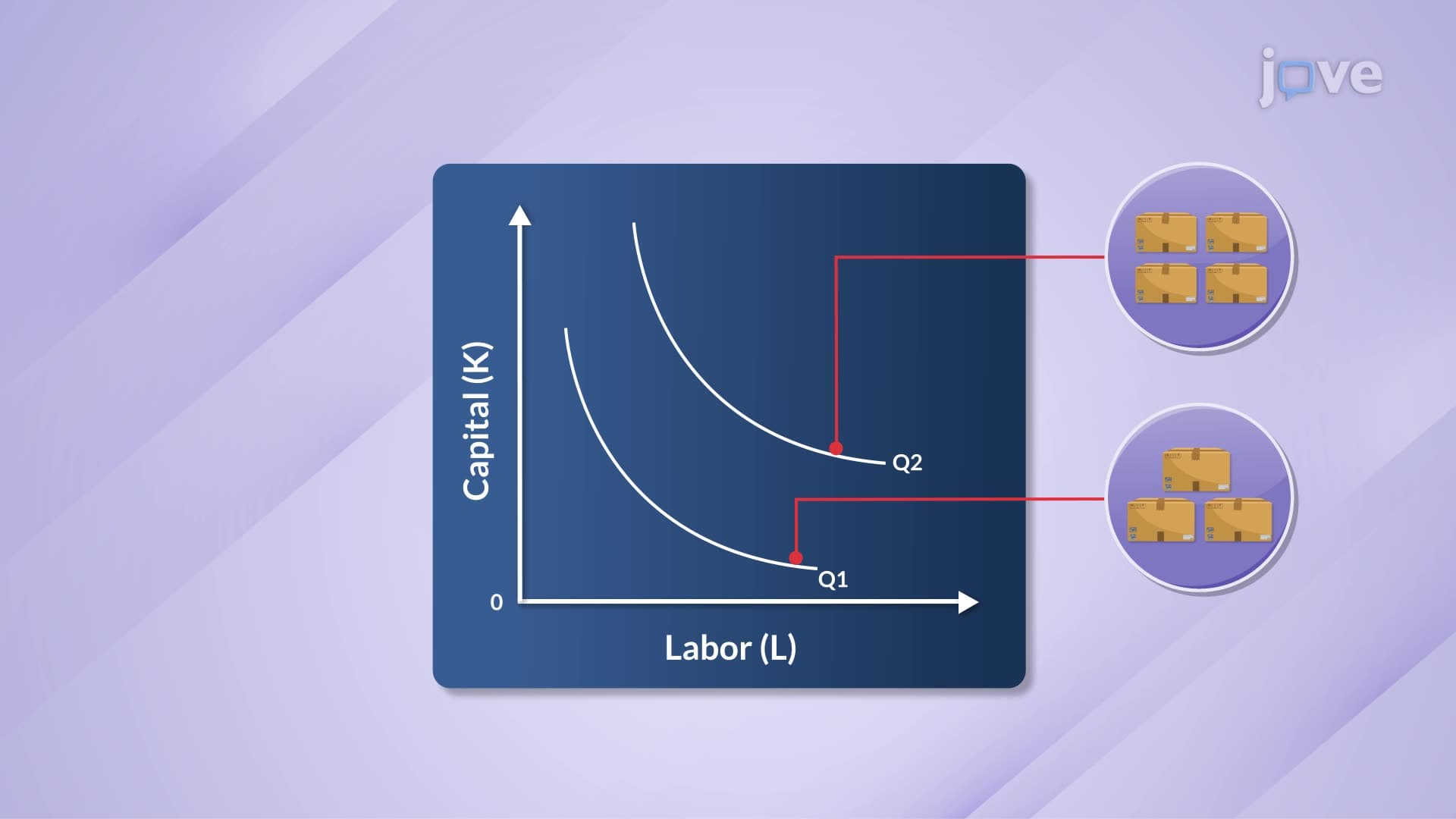
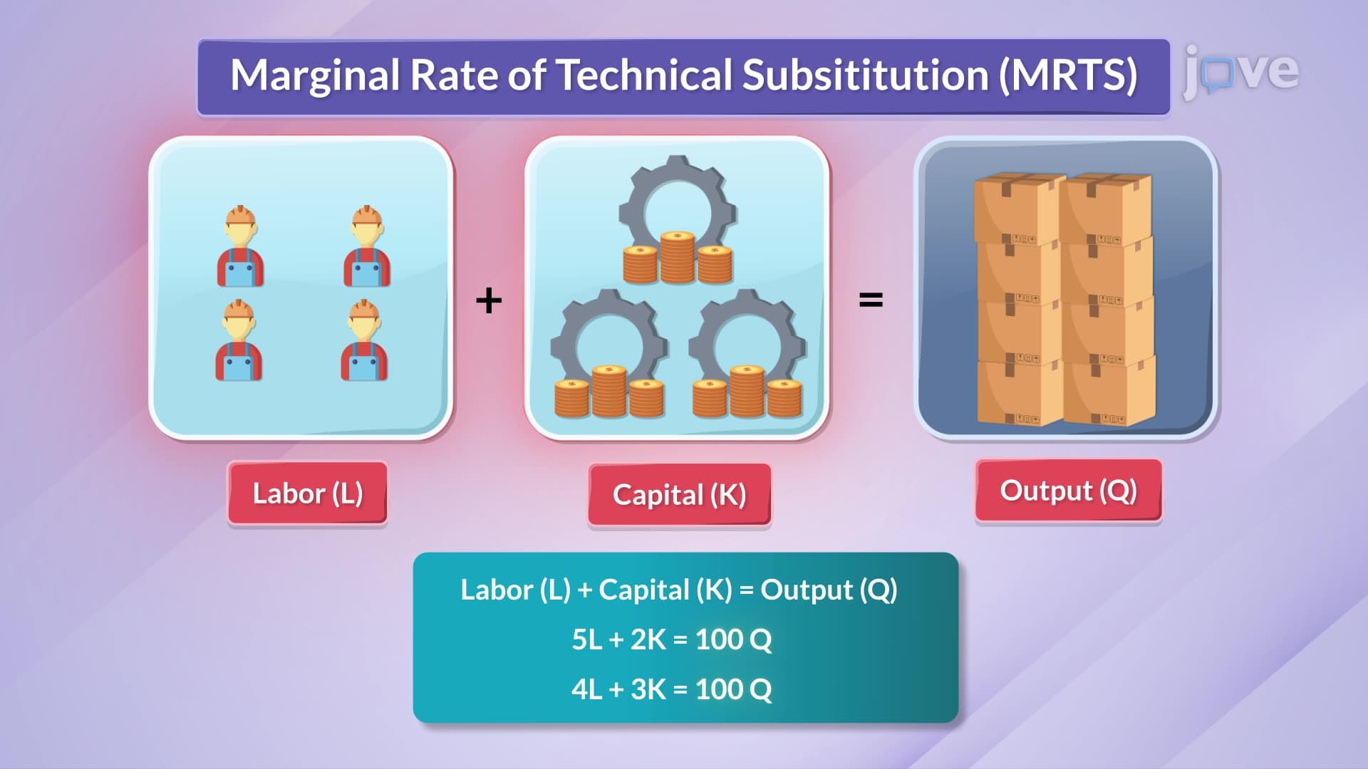
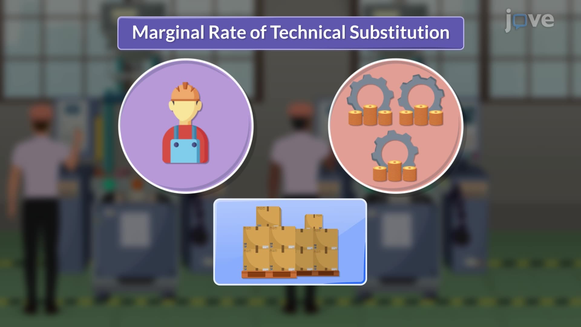
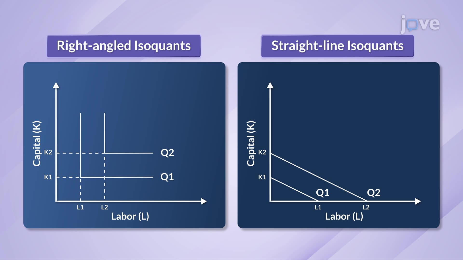
5. Isoquant Analysis and Input Substitution Isoquants represent all possible labor-capital combinations producing identical output levels, similar to how indifference curves work in consumer theory. A car wash business might achieve 100 daily services using either many hand-washers with minimal equipment or fewer workers with advanced automated systems. The curved shape reflects diminishing marginal rate of technical substitution-initially, many workers can replace one machine, but this rate decreases as substitution continues. This analysis helps firms like General Motors evaluate different production technologies and input mixes.
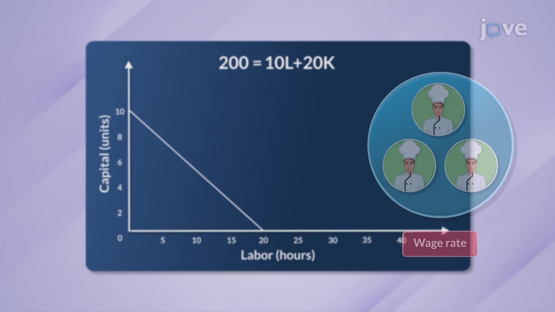
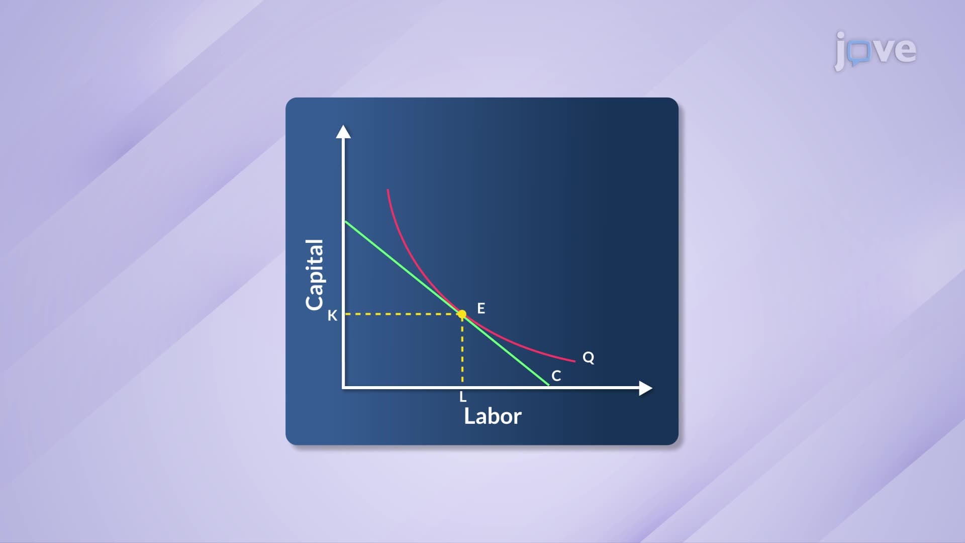
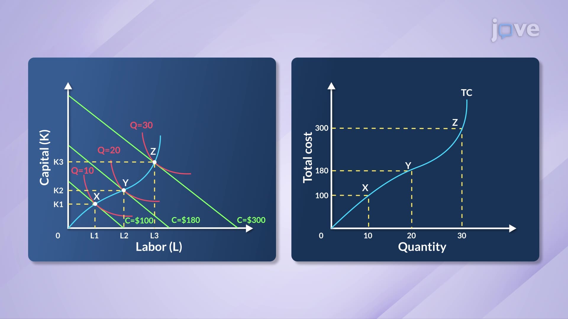
6. Cost Minimization Through Isocost Analysis Isocost lines show all input combinations a firm can afford within a specific budget, with slope reflecting relative input prices. When wage rates increase, the line becomes steeper, indicating labor has become relatively more expensive than capital. A restaurant chain like Chipotle facing rising minimum wages might substitute toward more automated food preparation equipment. The tangency point between isoquant and isocost lines reveals the cost-minimizing input combination, where the marginal rate of technical substitution equals the input price ratio.
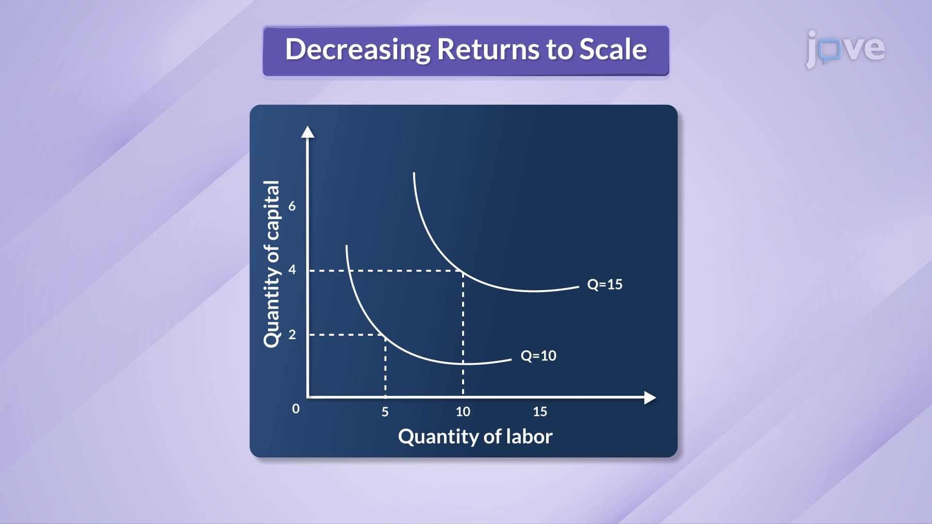
7. Returns to Scale in Production Returns to scale describe how output changes when all inputs increase proportionally. Increasing returns occur when doubling inputs more than doubles output, often due to specialization benefits-a large electronics manufacturer like Apple can dedicate workers to specific assembly tasks, improving efficiency. Decreasing returns happen when output increases less than proportionally, typically from management difficulties in large organizations. Constant returns mean proportional input and output changes. Understanding these patterns helps firms determine optimal size and expansion strategies across different industries.
8. Technological Change and Productivity Technological advancement allows firms to produce the same output using fewer inputs, shifting isoquants inward toward the origin. When Amazon introduced warehouse robots, the same fulfillment capacity required fewer workers and less floor space. Some technologies are capital-biased (favoring machinery) while others are labor-biased (enhancing worker productivity). The US manufacturing sector exemplifies this through automation adoption, where companies maintain production levels while reducing traditional input requirements, demonstrating total factor productivity improvements that drive economic growth.
