Market Equilibrium

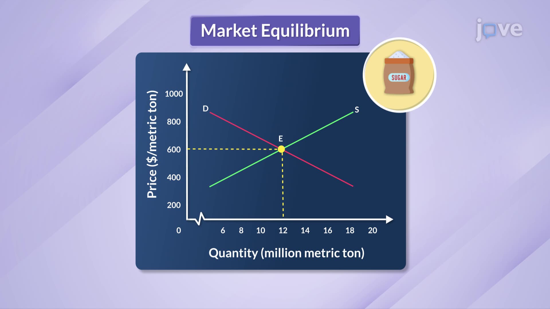
Market equilibrium occurs when supply and demand curves intersect, determining the price and quantity where markets clear. This JoVE Coach course explores equilibrium dynamics through practical US examples like sugar and bicycle markets, examining how shifts in supply and demand affect prices, quantities, and market outcomes including shortages, surpluses, and price adjustments during emergencies.

• Understand how market equilibrium is determined through the intersection of supply and demand curves
• Identify equilibrium price and quantity using mathematical equations and graphical analysis
• Analyze the causes and effects of market shortages and surpluses on consumer and producer behavior
• Explore how shifts in demand curves impact equilibrium price and quantity in real markets
• Examine the effects of supply curve shifts on market outcomes and pricing decisions
• Apply concepts to simultaneous shifts in both demand and supply curves moving in the same direction
• Understand market dynamics when demand and supply shift in opposite directions
• Evaluate price gouging scenarios and their relationship to supply demand equilibrium during emergencies

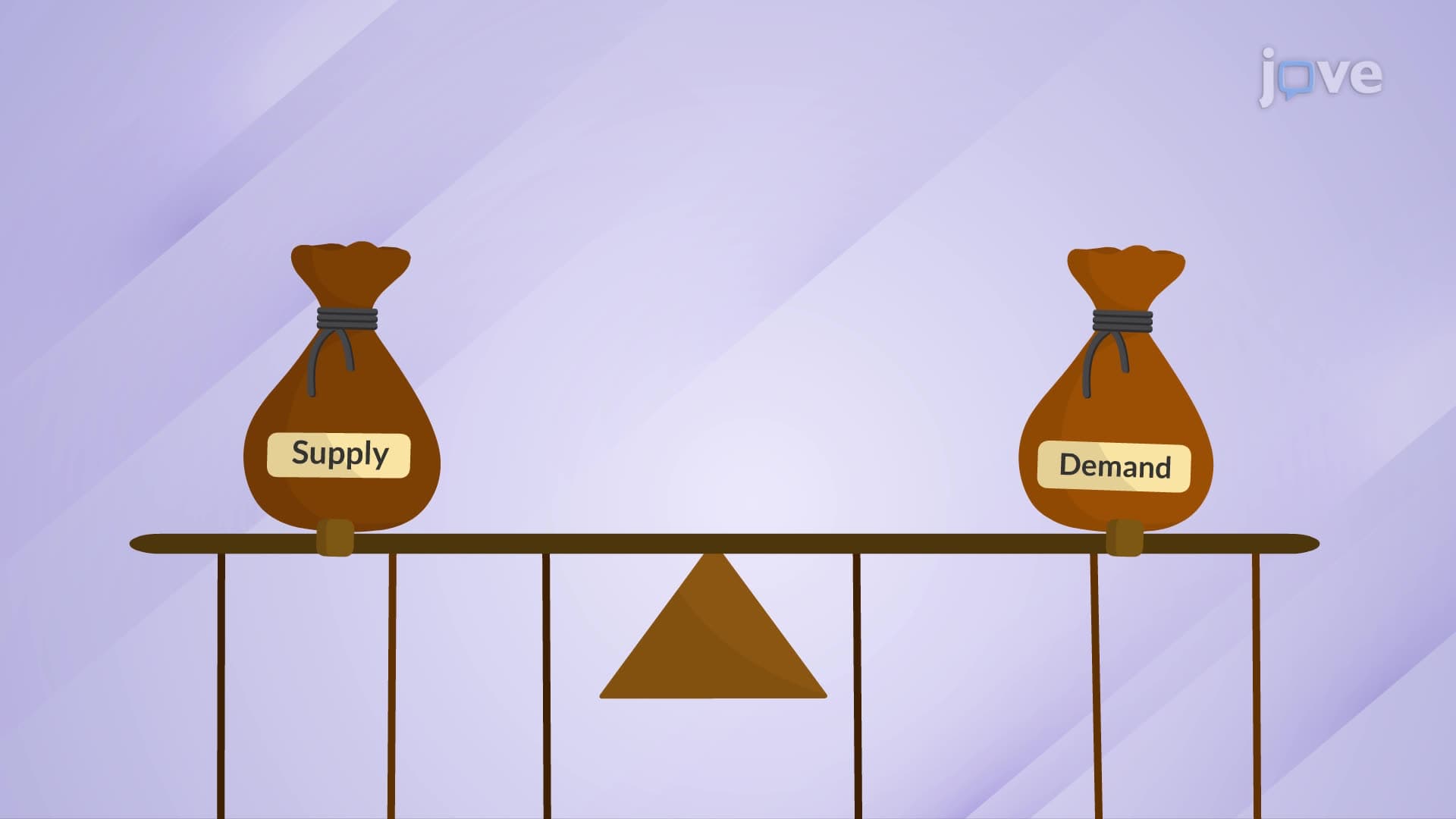
1. Fundamentals of Market Equilibrium and Price Determination Market equilibrium represents the balance point where quantity supplied equals quantity demanded, creating the market-clearing price. At this intersection, both buyers and sellers achieve satisfaction - consumers purchase desired quantities while producers sell their intended output. Using the US sugar market example, when supply and demand curves meet at $600 per ton with 12 million metric tons traded, this establishes equilibrium. The market-clearing mechanism ensures efficient resource allocation, as any deviation from equilibrium triggers natural corrective forces that restore balance through price adjustments.

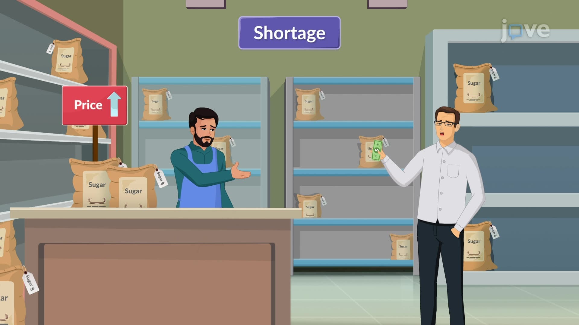
2. Understanding Market Imbalances: Shortages and Surpluses Market disequilibrium creates either shortages or surpluses that activate self-correcting mechanisms. Shortages occur when demand exceeds supply at current prices, like sugar priced below equilibrium at $400 per ton, causing buyers to compete and bid prices upward. Surpluses develop when supply exceeds demand, such as sugar priced above equilibrium at $800 per ton, forcing sellers to reduce prices to clear inventory. These imbalances naturally resolve through price adjustments, demonstrating how competitive markets maintain stability and efficient resource distribution.

3. Mathematical Models for Equilibrium Analysis How market equilibrium is determined mathematically involves setting quantity demanded equal to quantity supplied using linear equations. For the sugar market example, if Qd = 20 - 0.013P and Qs = -8 + 0.033P, equilibrium occurs where 20 - 0.013P = -8 + 0.033P, solving for P = $600. Substituting back yields equilibrium quantity of 12 million metric tons. This mathematical approach provides precise equilibrium calculations, enabling economists and businesses to predict market outcomes and make informed pricing decisions based on quantitative analysis.

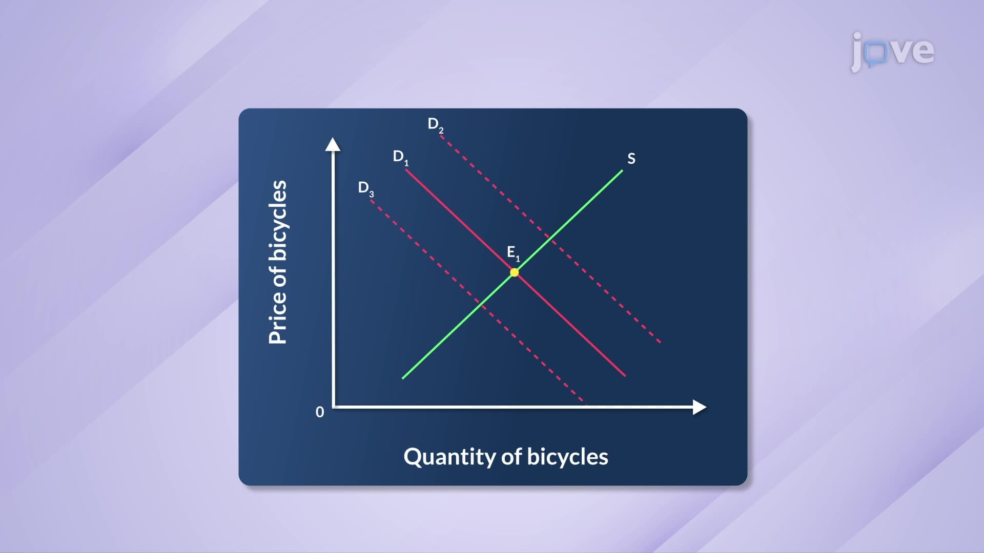
4. Demand Shifts and Market Adjustments Demand curve shifts significantly impact equilibrium price and quantity while supply remains constant. In US bicycle markets, fitness trends increasing cycling popularity shift demand rightward, creating shortages at original prices and driving both price and quantity higher. Conversely, safety concerns shifting demand leftward create surpluses, reducing both equilibrium price and quantity. These shifts demonstrate how external factors like consumer preferences, income changes, or social trends influence market outcomes, requiring businesses to adapt pricing and production strategies accordingly.

5. Supply Changes and Economic Impacts Supply curve shifts affect equilibrium through production cost changes, technology improvements, or regulatory modifications. Government subsidies for US bicycle manufacturing shift supply rightward, creating surpluses that reduce prices while increasing quantities sold. Alternatively, steel shortages shift supply leftward, causing shortages that raise prices and decrease quantities. These examples illustrate how production factors, resource availability, and government policies influence market equilibrium, affecting both consumer welfare and producer profitability across different economic sectors.

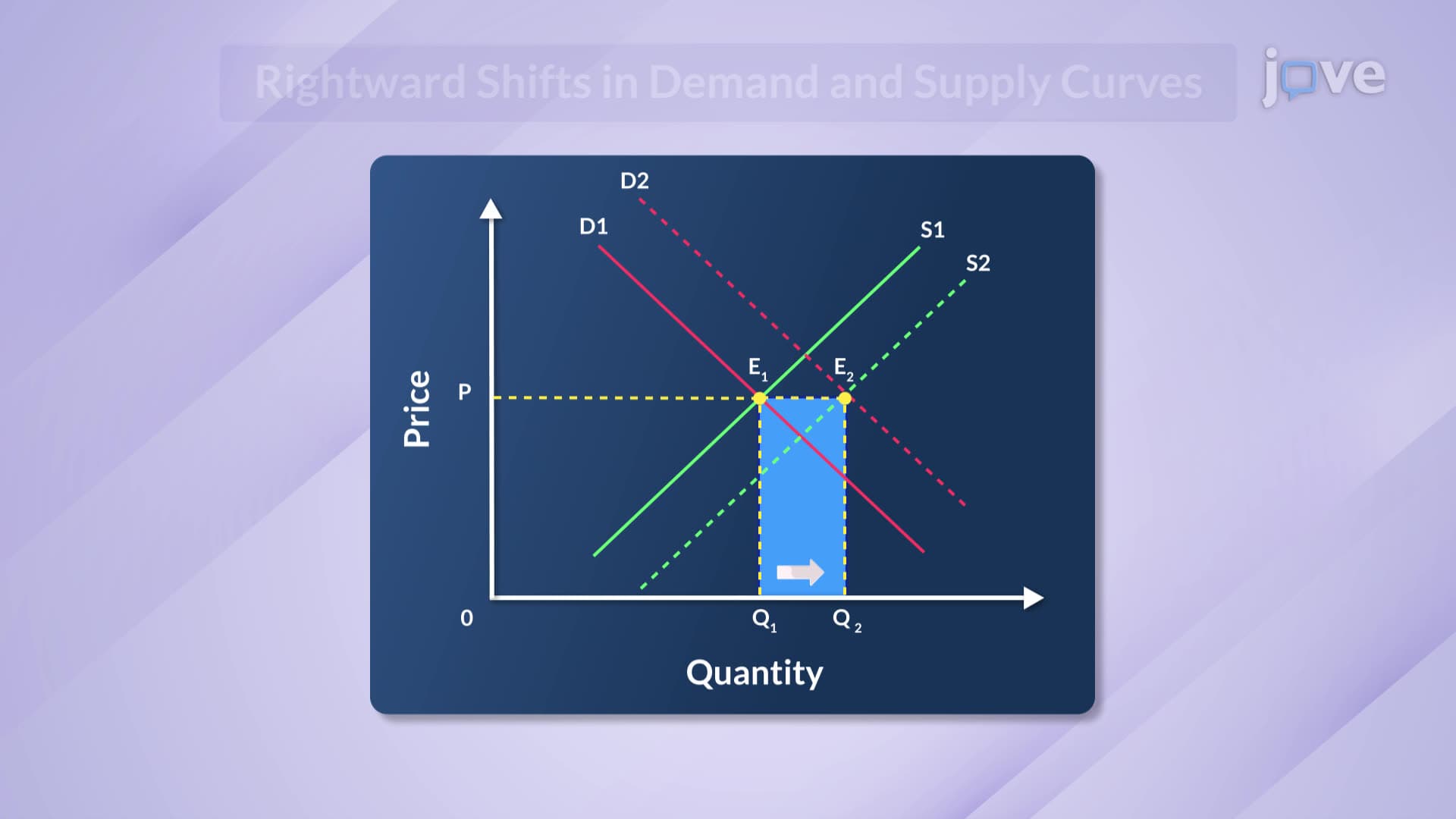
6. Simultaneous Market Shifts in Same Direction When demand and supply curves shift simultaneously in the same direction, equilibrium quantity changes predictably while price effects depend on relative shift magnitudes. During economic prosperity in US automobile markets, increased consumer confidence shifts demand right while manufacturing improvements shift supply right, definitively increasing equilibrium quantity. However, equilibrium price may rise, fall, or remain constant depending on whether demand or supply shifts more significantly, requiring careful analysis of both market forces.

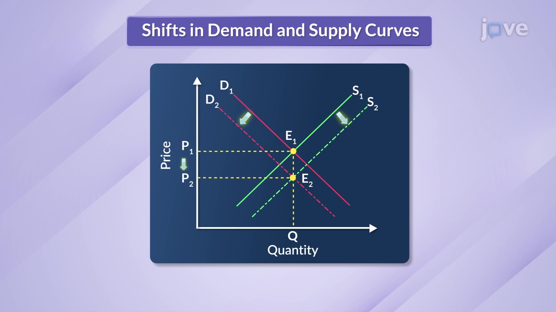
7. Opposite Direction Market Shifts and Price Effects Simultaneous opposite shifts create definite price changes while quantity effects remain uncertain. In gasoline car markets, improved fuel efficiency technology increases demand (rightward shift) while environmental regulations increase production costs, decreasing supply (leftward shift). This combination guarantees higher equilibrium prices as reduced supply cannot meet increased demand. The quantity effect depends on relative shift magnitudes, demonstrating complex market interactions requiring sophisticated analysis to predict outcomes accurately.

8. Price Gouging and Emergency Market Dynamics Emergency situations disrupt normal supply demand equilibrium, often leading to price gouging when sellers exploit sudden demand spikes or supply shortages. After natural disasters like tornadoes, water demand skyrockets while supply may be limited, causing prices to jump from $1 to $10 per bottle. While higher prices can help ration scarce resources and prevent hoarding, they disproportionately burden lower-income consumers. Many US states have implemented anti-price gouging laws to protect consumers during emergencies while maintaining market function.