Supply and its Elasticities

Supply elasticity measures how responsive producers are to price changes in the market. This comprehensive course through JoVE Coach explores the fundamental concepts of supply theory, including the law of supply, market dynamics, and price elasticity of supply calculations. Students will examine real-world applications using American industries like smartphone manufacturing, automotive production, and food service to understand how supply responds to price changes and various market factors affecting production decisions.

• Understand the basic definition of supply and the law of supply in economic theory
• Identify key factors that shift supply curves, including input costs, technology, and market expectations
• Learn to calculate market supply by combining individual producer supply schedules
• Analyze how input prices, technological advances, and seller numbers impact supply decisions
• Explore the mathematical representation of supply curves using linear functions
• Apply the percentage method to calculate price elasticity of supply (PES)
• Understand the five degrees of supply elasticity from perfectly elastic to perfectly inelastic
• Examine real-world examples from American industries to reinforce theoretical concepts

1. Supply Fundamentals and the Law of Supply Supply represents the quantity of goods producers are willing and able to offer at various price levels during a specific time period. The law of supply establishes a positive relationship between price and quantity supplied - as prices increase, producers supply more goods to maximize profits. This relationship appears graphically as an upward-sloping supply curve. For example, when gasoline prices rise in Texas, oil companies increase production and refining capacity. The law assumes all other factors remain constant (ceteris paribus), allowing economists to isolate the price-quantity relationship from other market influences like production costs or technological changes.

2. Mathematical Representation of Supply Curves Supply curves can be expressed mathematically using linear functions: Qs = mP + b, where Qs represents quantity supplied, m shows the slope (quantity change per price unit), P is price, and b represents the y-intercept. For instance, if a California vineyard supplies 500 additional bottles for every $1 price increase, starting from zero at $5, the function becomes Qs = 500P - 2500. The inverse supply function (P = Qs/500 + 5) reveals the supply choke price - the minimum price needed for any production. This mathematical approach helps predict producer behavior and market responses to price fluctuations.

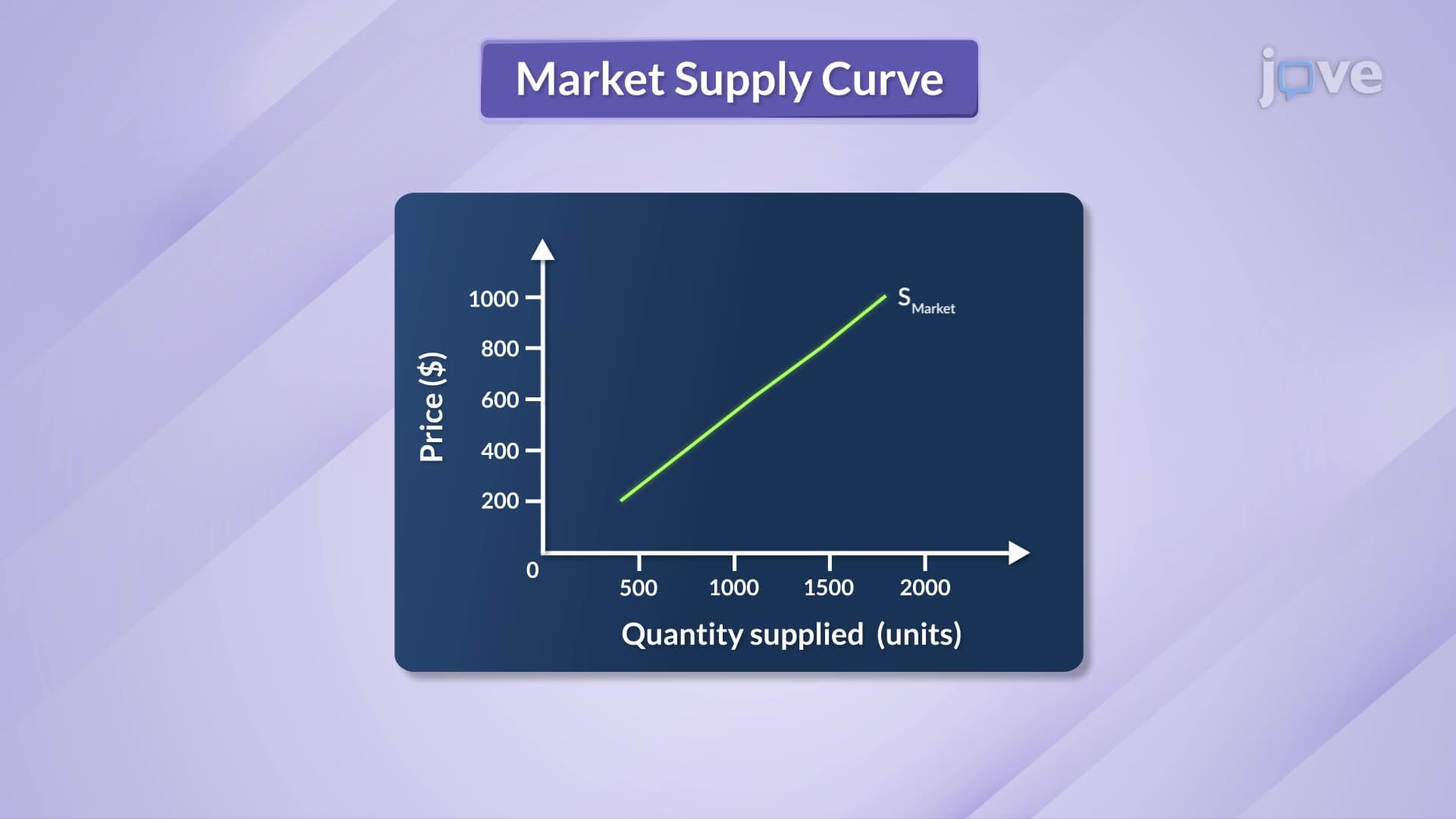
3. Market Supply and Individual Producer Aggregation Market supply combines all individual producers' supply schedules within a specific market. For example, the total smartphone supply in the US market represents the combined output from Apple, Samsung, Google, and other manufacturers at various price points. Graphically, market supply curves are created by horizontally adding individual supply curves. If Producer A supplies 100 units at $10 and Producer B supplies 150 units at the same price, market supply equals 250 units at $10. This aggregation process helps economists understand overall market capacity and predict how collective producer behavior responds to price changes across entire industries.

4. Factors Affecting Supply: Input Prices and Technology Input prices significantly impact supply decisions by affecting production costs. When steel prices increase, automobile manufacturers in Detroit face higher production costs, potentially reducing vehicle supply (leftward supply curve shift). Conversely, decreased labor costs can increase supply (rightward shift). Technological advancement typically increases supply by improving efficiency and reducing per-unit costs. For example, robotic assembly lines in American automotive plants have dramatically increased production capacity while lowering costs. However, some technologies increase costs - like emissions control systems that comply with EPA regulations - which can decrease supply despite being technologically advanced.

5. Market Expectations and Number of Sellers Producer expectations about future prices influence current supply decisions. If furniture manufacturers anticipate higher wood prices next quarter, they might reduce current supply to sell more later at higher prices (leftward shift). Conversely, expecting future price declines encourages increased current production (rightward shift). The number of market sellers directly affects total supply. When new craft breweries enter markets like Colorado or Oregon, beer supply increases (rightward shift). Market exits decrease supply (leftward shift). These dynamics are particularly visible in emerging industries like renewable energy, where new companies entering solar panel manufacturing significantly impact market supply.

6. Price Elasticity of Supply Calculation and Interpretation Price elasticity of supply (PES) measures supply responsiveness to price changes using the formula: PES = (% Change in Quantity Supplied) / (% Change in Price). If a bakery increases donut production from 1,000 to 1,200 units when prices rise from $1.00 to $1.20, the calculation shows: (200/1000 × 100) / (0.20/1.00 × 100) = 20%/20% = 1.0. This unitary elasticity means quantity supplied changes proportionally with price. Values greater than 1 indicate elastic supply (highly responsive), while values less than 1 show inelastic supply (less responsive). Understanding PES helps businesses make production decisions and governments predict policy impacts.

7. Degrees of Supply Elasticity Supply elasticity ranges across five categories. Perfectly elastic supply (PES = ∞) shows horizontal supply curves where small price changes cause infinite quantity changes - theoretical in most real markets. Relatively elastic supply (PES > 1) features flatter curves where producers respond strongly to price changes, like seasonal agricultural products. Unitary elastic supply (PES = 1) shows proportional responses. Relatively inelastic supply (0 < PES < 1) displays steeper curves where quantity changes less than proportionally to price, common with specialized manufacturing requiring significant lead times. Perfectly inelastic supply (PES = 0) shows vertical curves where quantity remains constant regardless of price - like original Picasso paintings or beachfront property in Malibu.