- Calculus
- Applications of Differentiation
Micro-courses:15

Applications of Differentiation
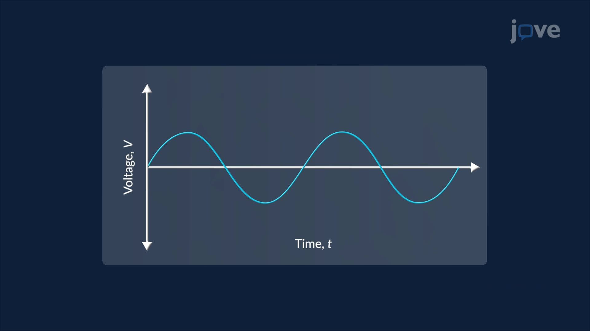
1. Absolute and Local Extreme Values
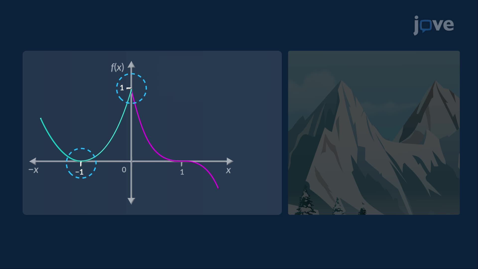
2. Critical Numbers and the Closed Interval Method
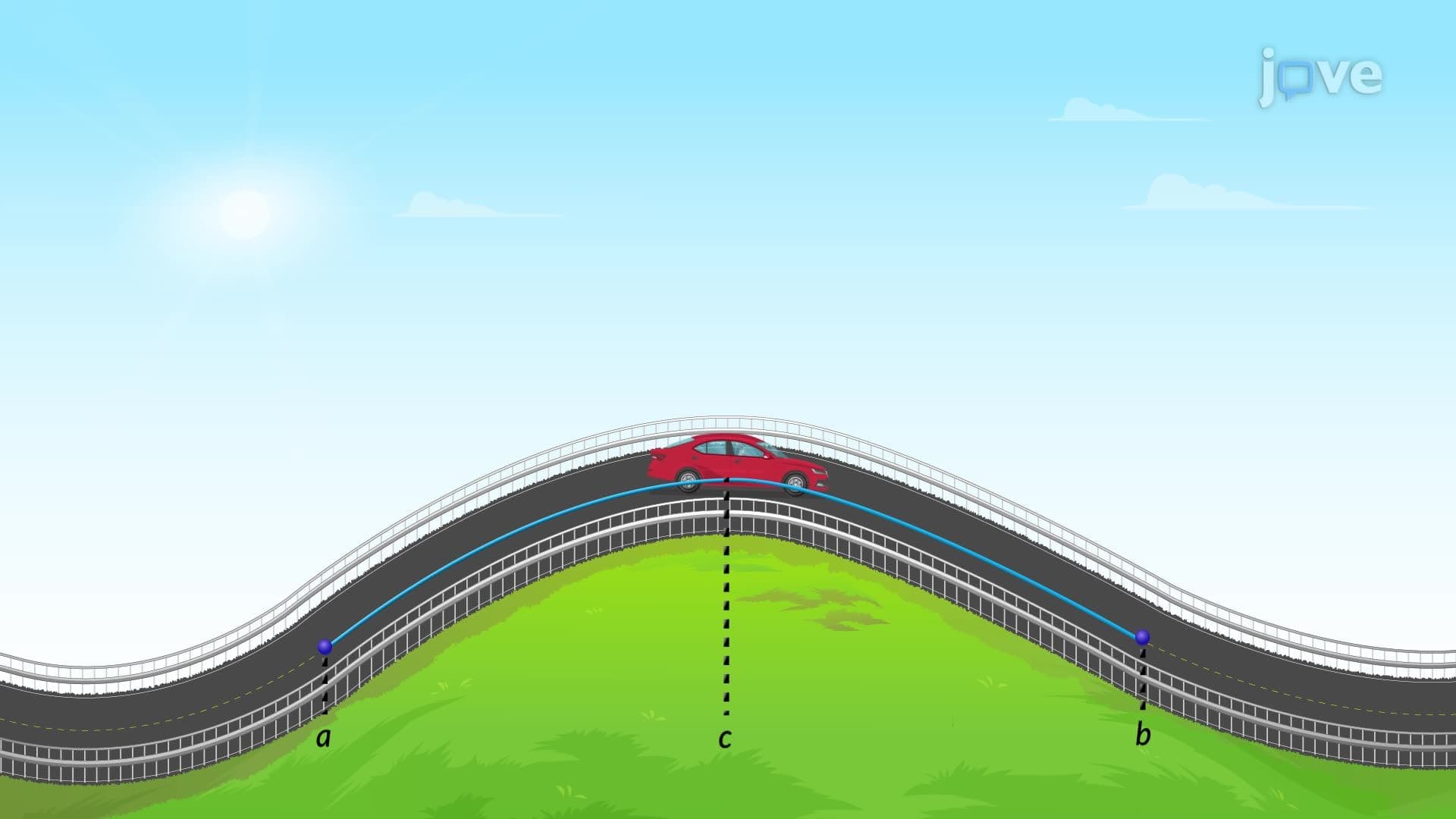
3. Rolle’s Theorem
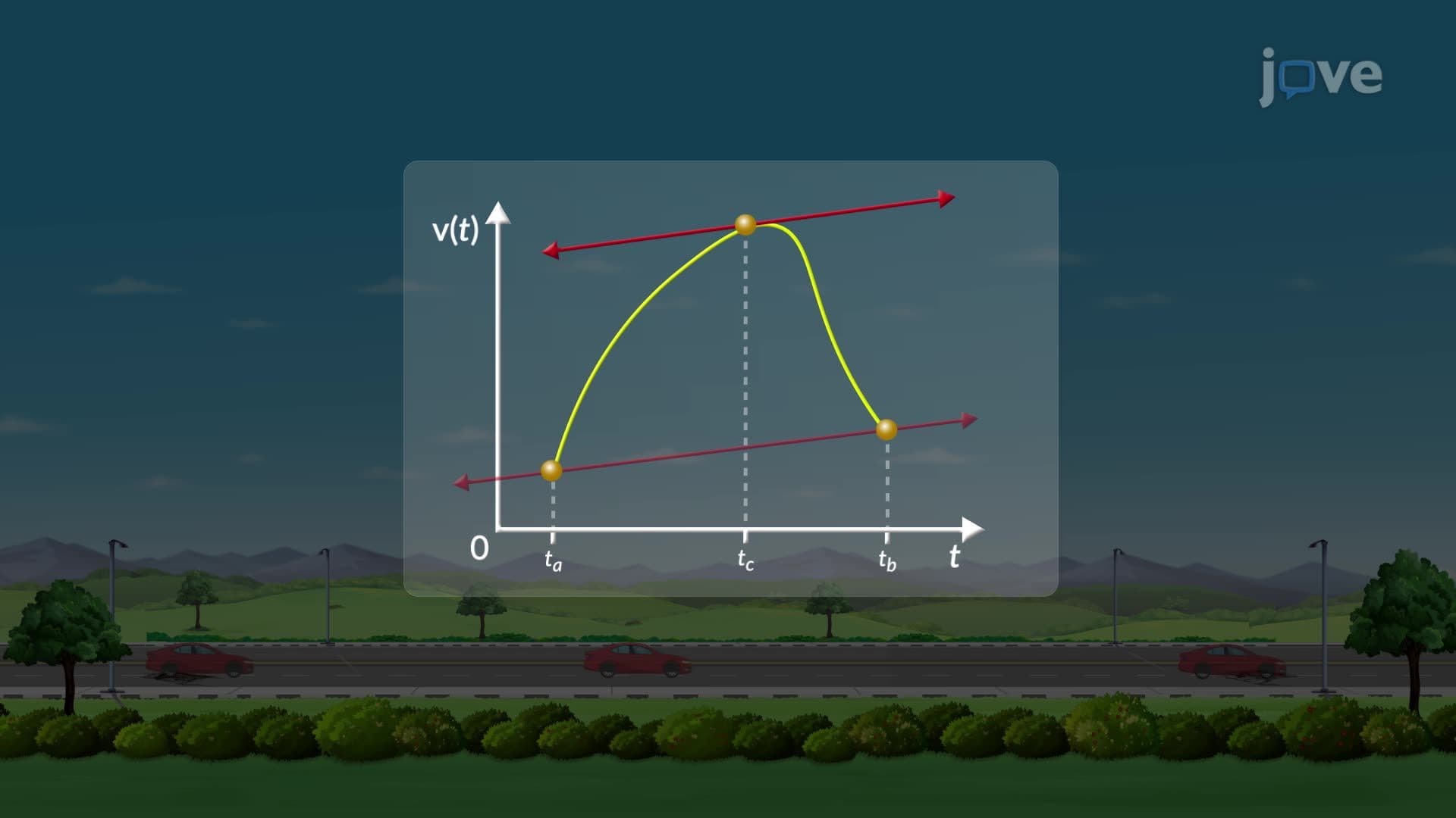
4. The Mean Value Theorem
5. First Derivatives and the Shape of a Graph
6. First Derivative Test: Problem Solving
7. Second Derivatives and the Shape of a Graph
8. Second Derivative Test: Problem Solving
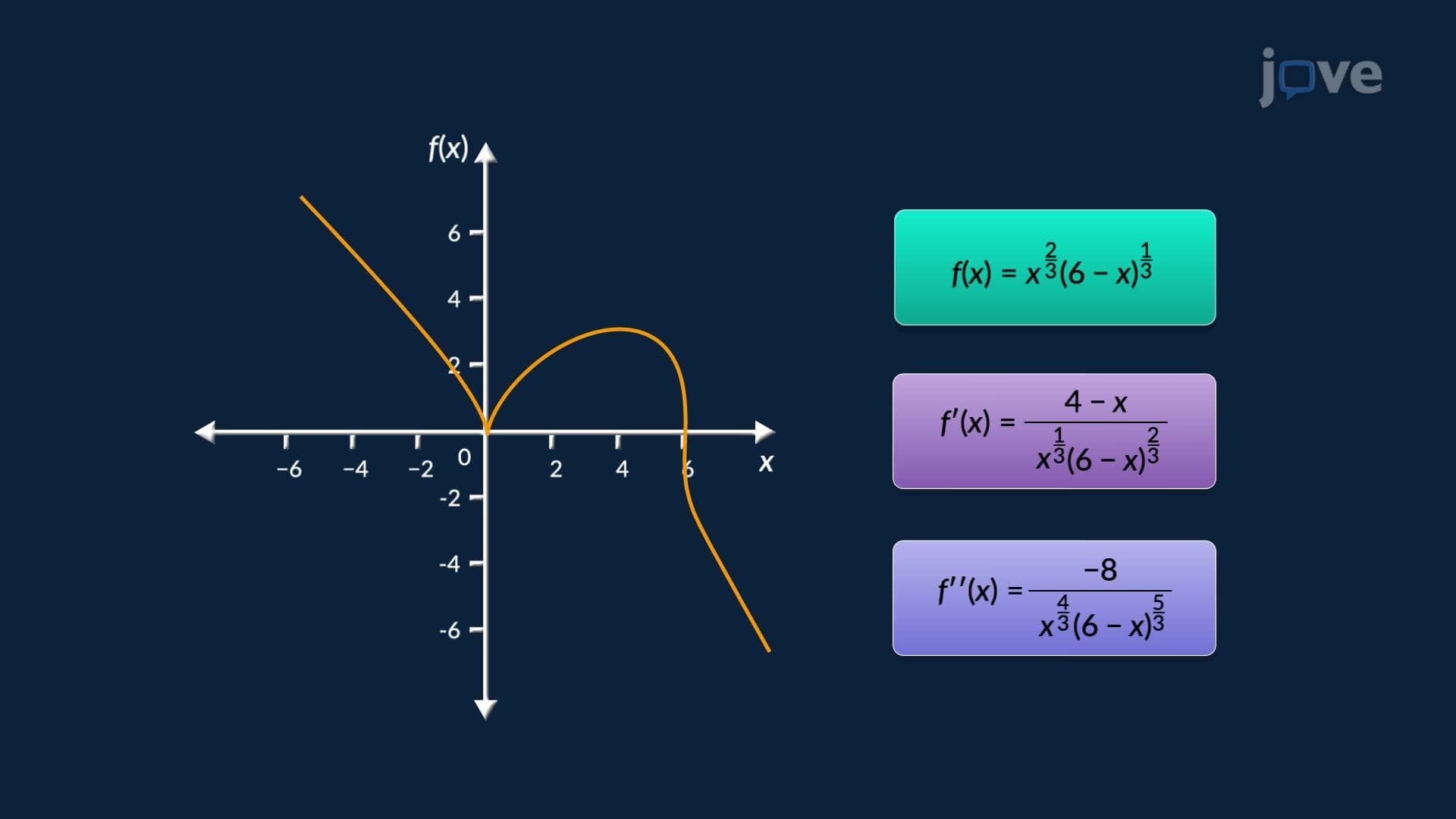
9. Curve Sketching and Derivatives

10. Indeterminate Forms and L’Hôpital’s Rule

11. Indeterminate Products
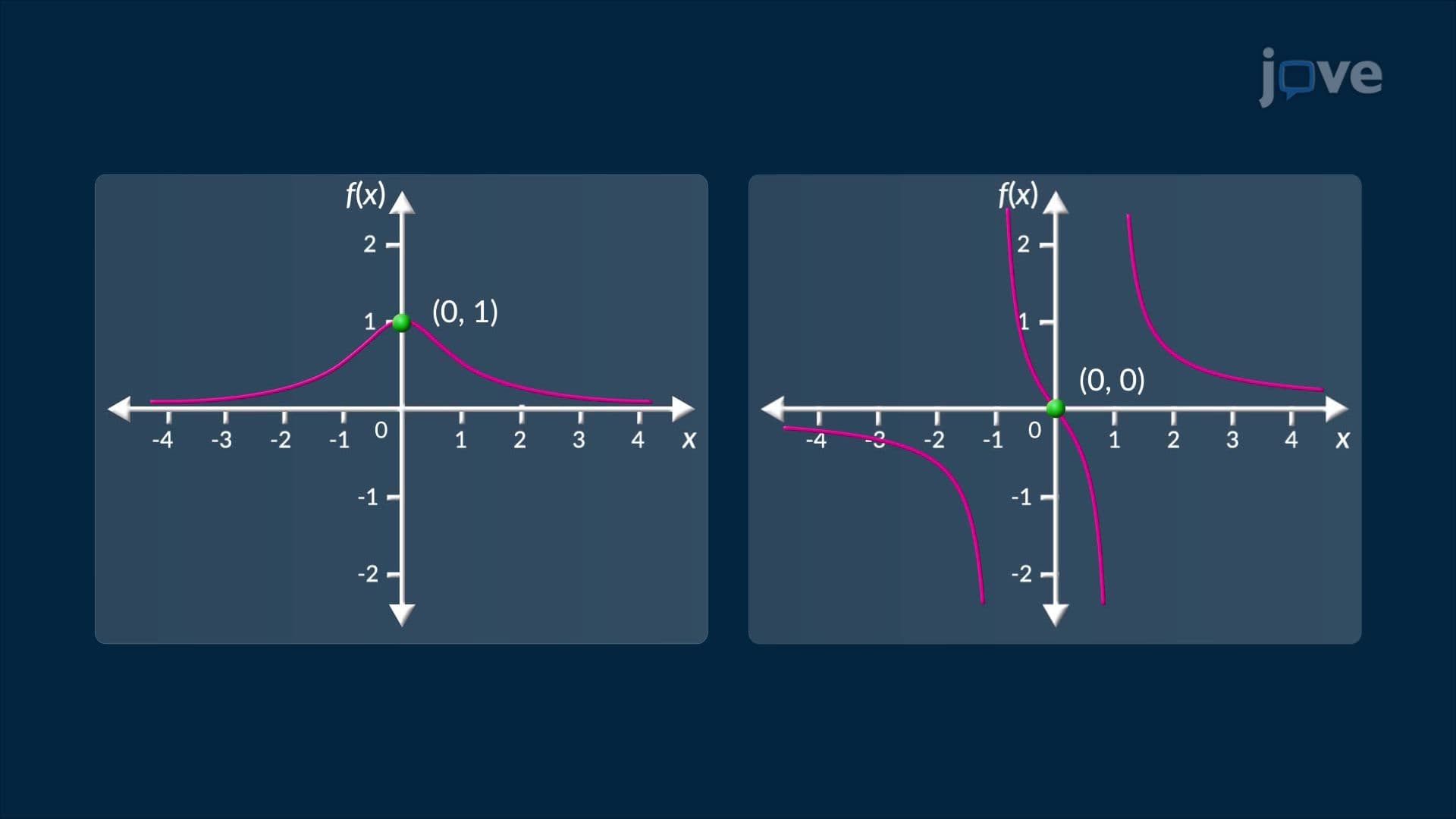
12. Guidelines for Sketching a Curve
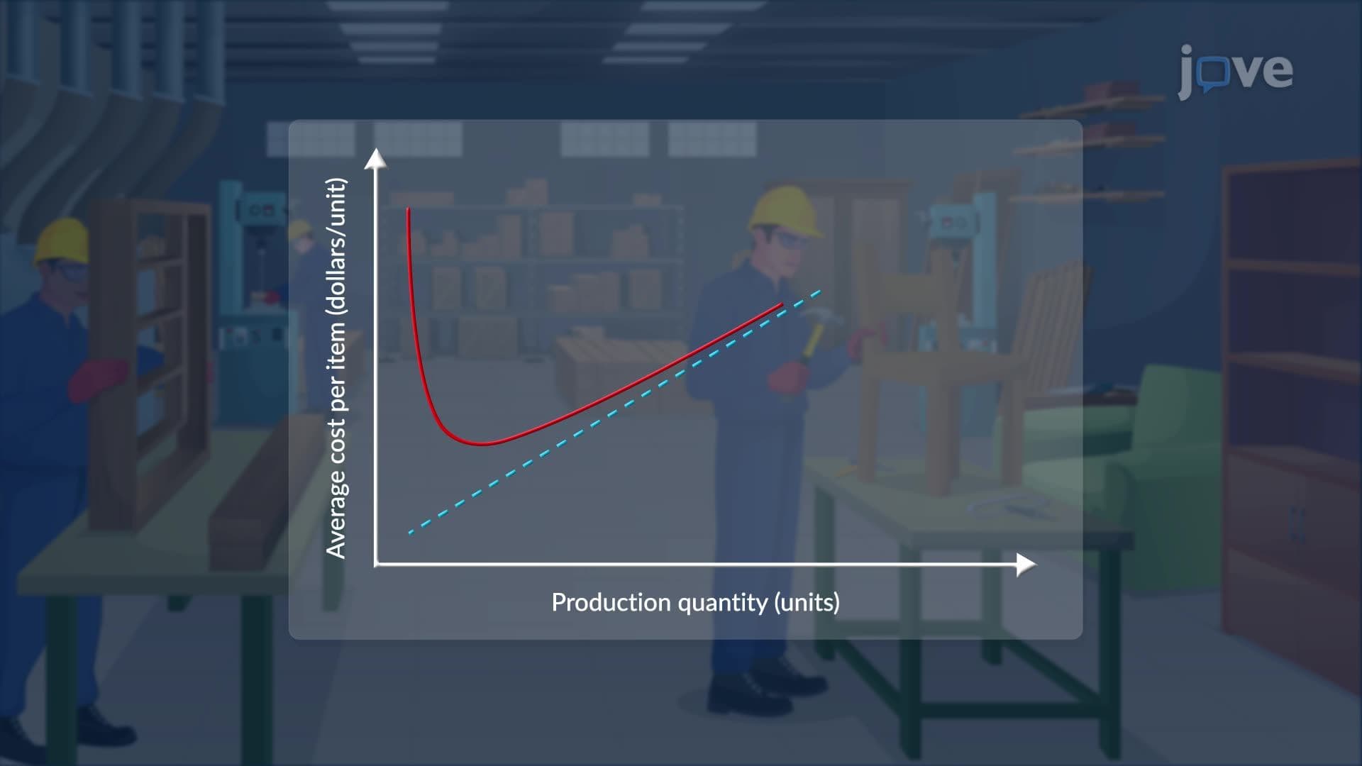
13. Slant Asymptotes

14. Optimization Problems

15. Application of Differentiation to Business

16. Newton’s Method

17. The Antiderivative of a Function
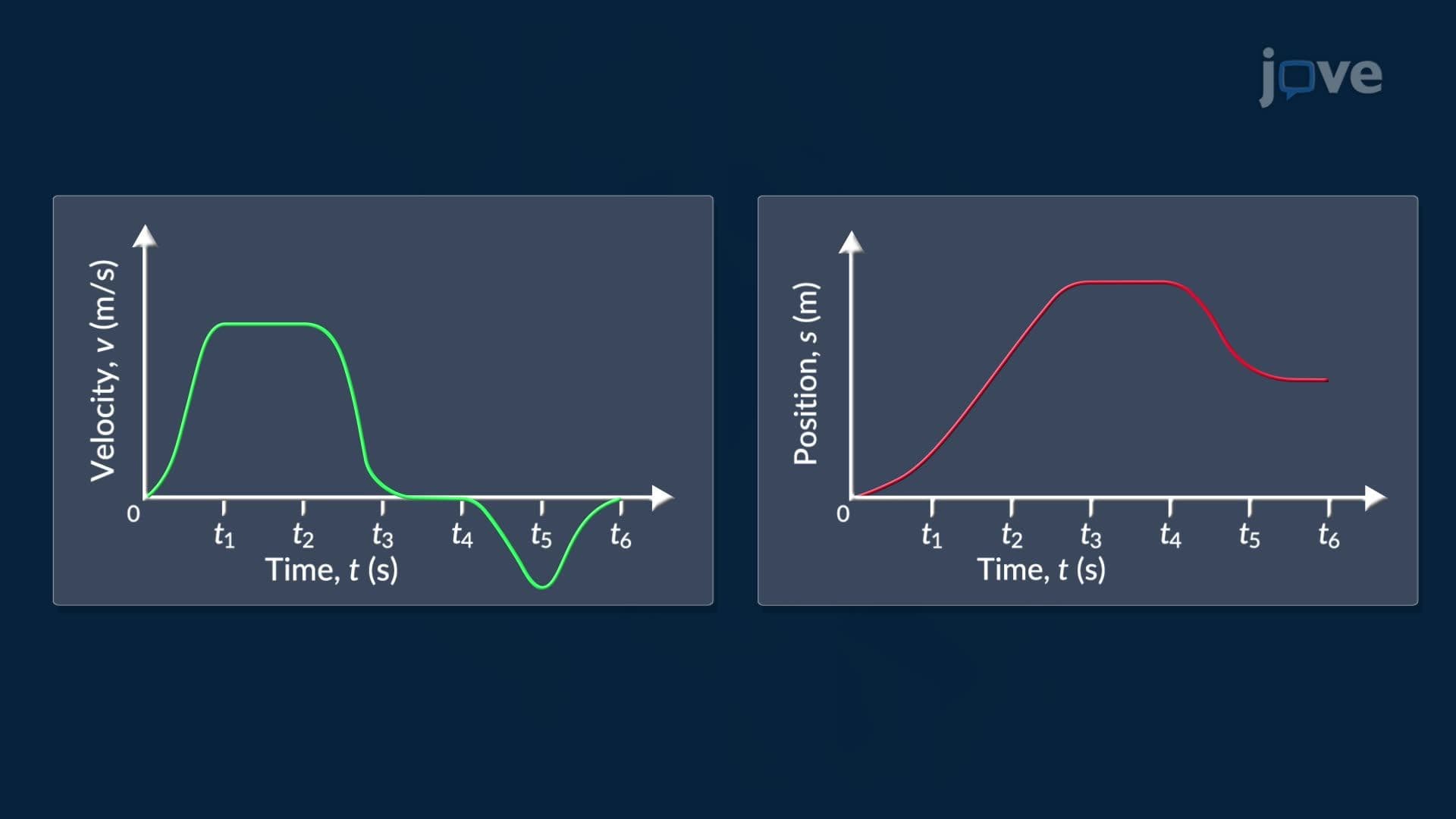
18. Graphing Antiderivatives

19. Application of Antiderivatives: Linear Motion
Differentiation Applications explores how derivatives solve real-world problems across science, engineering, business, and medicine. Powered by JoVE Coach, this micro-course covers optimization problems, curve sketching, the Mean Value Theorem, L'Hôpital's Rule, and antiderivatives. Students learn how to use differentiation to find maximum and minimum values, analyze graph behavior, model linear motion, and apply Newton's Method to complex equations arising in US academic and professional contexts.
- Understand the Extreme Value Theorem and how absolute and local extrema are identified on closed intervals
- Learn how Rolle's Theorem and the Mean Value Theorem relate instantaneous and average rates of change
- Identify critical numbers, inflection points, and concavity using first and second derivative tests
- Apply optimization problems to real scenarios such as maximizing revenue, minimizing cost, and solving geometric constraints
- Explore curve sketching techniques including slant asymptotes, intercepts, symmetry, and limiting behavior
- Analyze indeterminate forms using L'Hôpital's Rule for limits involving zero over zero or infinity over infinity
- Apply Newton's Method as an iterative tool for approximating roots of nonlinear equations
- Understand antiderivatives and their applications to linear motion, including velocity and displacement problems
1. Absolute and Local Extreme Values The Extreme Value Theorem guarantees that any continuous function on a closed interval has both an absolute maximum and an absolute minimum. Local extrema occur at peaks and valleys within the interval, while absolute extrema represent the overall highest and lowest values. Real-world examples include identifying the highest and lowest temperatures over a 24-hour period or determining the safe voltage range in an alternating current circuit. These concepts underpin engineering safety standards and environmental data analysis across the United States.
2. Critical Numbers and the Closed Interval Method Critical numbers are domain values where the derivative equals zero or is undefined. Fermat's Theorem states that local extrema must occur at critical numbers, though not every critical number produces an extremum. The Closed Interval Method identifies absolute extrema in three steps: find critical numbers inside the open interval, evaluate the function at those points, and evaluate at both endpoints. Comparing all resulting values identifies the absolute maximum and minimum — an approach widely used in US engineering design and economic modeling.
3. Rolle's Theorem and the Mean Value Theorem Rolle's Theorem states that a function continuous on a closed interval, differentiable on the open interval, and equal at both endpoints must have at least one point inside where the derivative equals zero. The Mean Value Theorem extends this idea: if the same continuity and differentiability conditions hold, at least one interior point must exist where the instantaneous rate of change equals the average rate of change across the interval. These theorems are foundational in AP Calculus proofs and appear frequently in US university-level analysis courses.
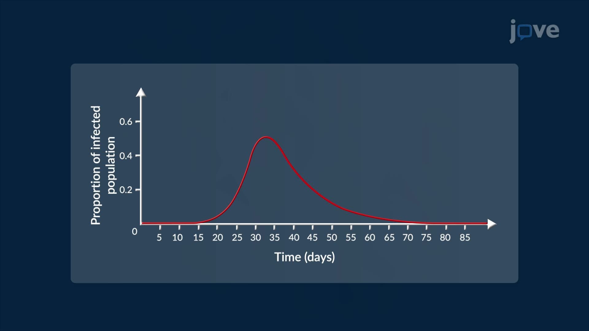
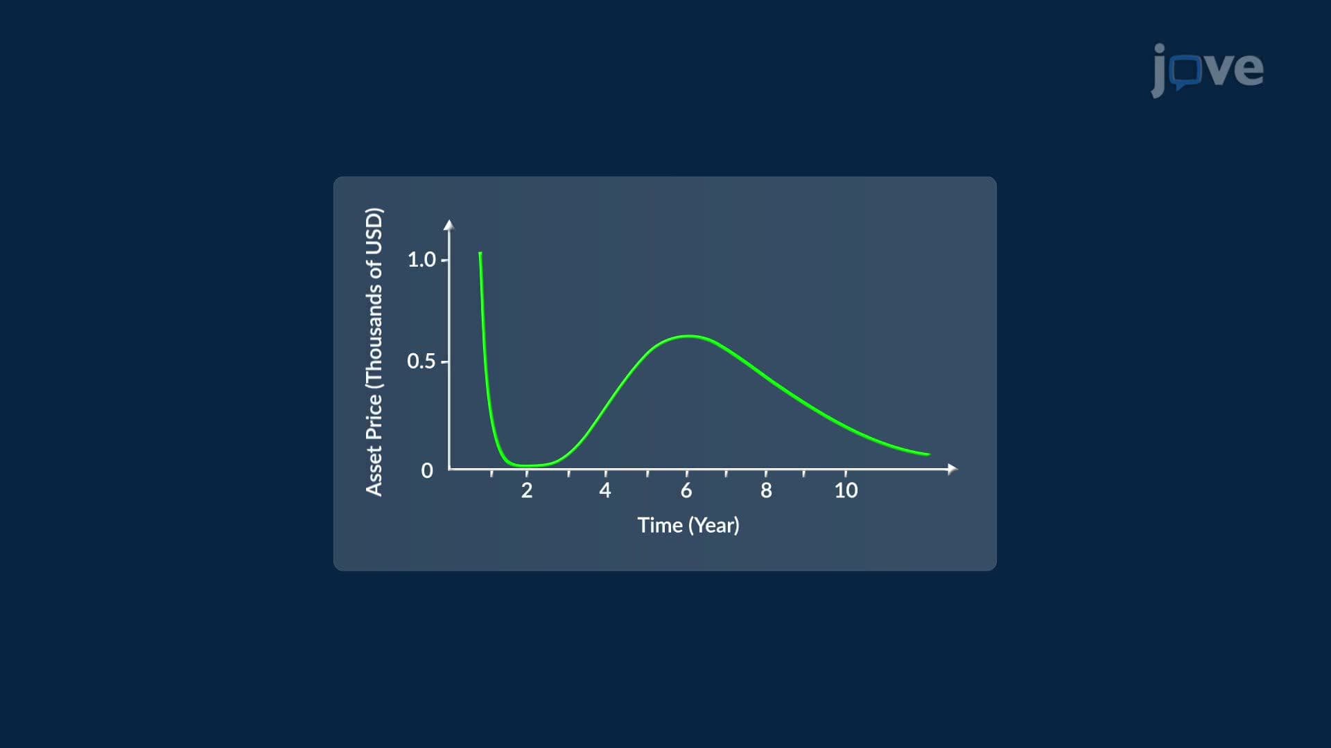
4. First Derivative Test and Graph Shape The first derivative reveals whether a function is increasing or decreasing at any point. A positive derivative indicates an upward-sloping graph; a negative derivative indicates a downward slope. At critical points, the sign change of the derivative determines whether a local maximum or minimum exists. If the sign shifts from positive to negative, the function reaches a local maximum; negative to positive indicates a local minimum. No sign change means neither extremum is present. Applications include tracking asset price movements in financial markets and modeling disease case counts during public health emergencies.
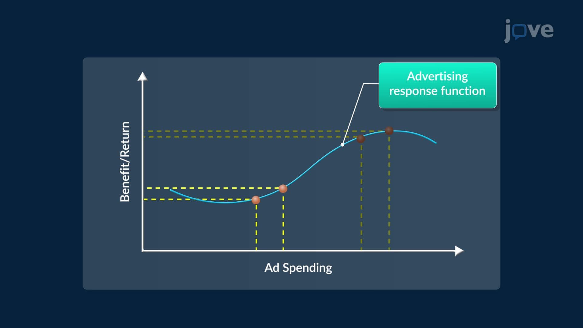
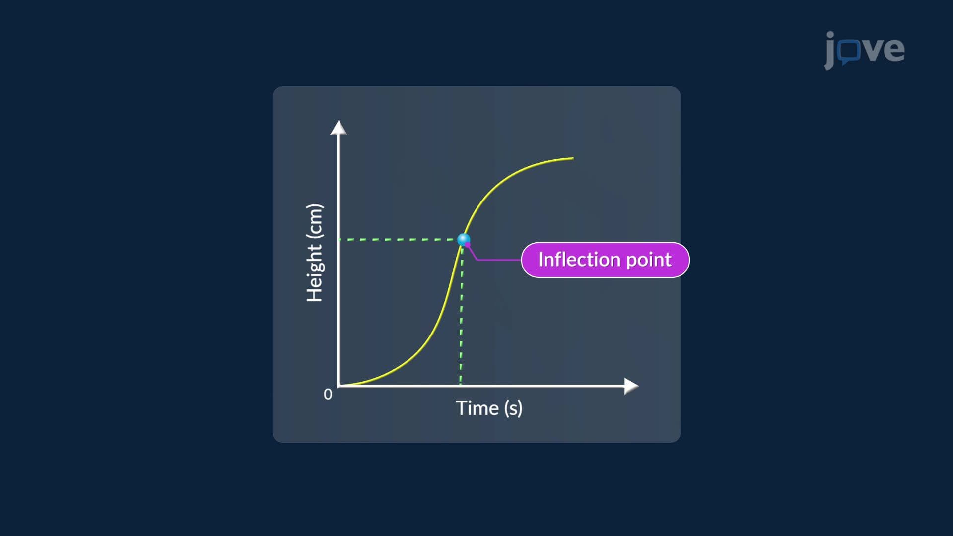
5. Second Derivative Test and Concavity The second derivative describes how the slope itself changes, revealing the curvature of a graph. A positive second derivative indicates a concave-up region where the graph bends upward; a negative second derivative signals a concave-down region. Inflection points occur where concavity changes direction, identified where the second derivative equals zero or is undefined. The second derivative test at critical points confirms whether each is a local maximum or minimum. In marketing analysis, concavity of an advertising-return curve tells businesses whether additional spending produces growing or diminishing returns.
6. Curve Sketching and Asymptotes Accurate curve sketching combines domain analysis, intercepts, symmetry, asymptote identification, and first and second derivative information. Vertical asymptotes occur where the denominator equals zero in rational functions. Slant asymptotes appear when the numerator's degree exceeds the denominator's by exactly one, found using polynomial long division. Horizontal asymptotes describe long-run behavior when degrees are equal or the denominator dominates. Together, these features enable accurate hand-drawn graphs — a skill tested on AP Calculus exams and essential for interpreting logistic growth models used in US epidemiology.
7. Indeterminate Forms and L'Hôpital's Rule Indeterminate forms such as zero over zero or infinity over infinity arise when direct substitution fails to resolve a limit. L'Hôpital's Rule states that, under appropriate differentiability conditions, the limit of a quotient equals the limit of the quotient of the derivatives. The process may be repeated if the indeterminate form persists. Indeterminate products — where one factor approaches zero and the other approaches infinity — can be rewritten as quotients before applying the rule. Real applications include modeling instantaneous bacterial growth rates from population data collected over shrinking time intervals in US biological research.
8. Optimization Problems Optimization uses derivatives to find the maximum or minimum value of a function subject to real-world constraints. Classic examples include maximizing a store's weekly revenue by identifying the ideal selling price for a product, or determining the longest rod that can navigate a right-angle corner between two hallways. The process involves writing an objective function, finding its critical numbers, and confirming the result using the first or second derivative test. Optimization problems appear extensively in AP Calculus, college engineering courses, and US business curricula, making them one of the highest-yield topics in applied calculus.
9. Newton's Method Newton's Method provides an iterative technique for approximating roots of equations that resist algebraic solutions. Starting from an initial estimate, a tangent line is drawn at that point, and its x-intercept becomes the next approximation. Each iteration applies the formula: new estimate equals the previous estimate minus the function value divided by its derivative at that point. Repeated application converges toward the actual root. Practical US applications include estimating interest rates on car loans described by nonlinear repayment equations — a scenario where standard algebra cannot isolate the variable but Newton's Method provides a precise numerical solution.
10. Antiderivatives and Linear Motion An antiderivative reverses differentiation, recovering an original function from its derivative. Because the derivative of any constant equals zero, a constant of integration C is always included to represent the full family of antiderivatives. In linear motion problems, integrating acceleration produces a velocity function, and integrating velocity produces a displacement function. Initial conditions — such as starting velocity or initial position — determine the value of C. A practical example involves calculating the braking distance of a car decelerating uniformly before reaching an obstacle 800 meters away, linking acceleration, velocity, and displacement through sequential integration.
Frequently Asked Questions
A local maximum is the highest function value in a small surrounding neighborhood — like the peak of a hill along a trail. An absolute maximum is the highest value over the entire domain or specified interval. A function can have several local maxima but only one absolute maximum on a closed interval. The Closed Interval Method finds the absolute extrema by comparing function values at all critical numbers and endpoints.
Both tests identify local extrema at critical numbers, but they work differently. The first derivative test checks how the sign of the derivative changes around a critical point and works even when the second derivative is zero or undefined. The second derivative test is faster — a positive second derivative confirms a local minimum, and a negative one confirms a local maximum — but it fails when the second derivative equals zero, requiring a return to the first derivative test. Using both gives a more complete picture of a function's behavior.
Differentiation applications are among the most heavily tested topics on both AP Calculus AB and BC. The AP exam includes free-response and multiple-choice questions on finding absolute and local extrema, applying the Mean Value Theorem, sketching curves using derivative information, solving optimization problems, and analyzing concavity and inflection points. BC students additionally encounter L'Hôpital's Rule. The College Board's course framework explicitly lists these as major learning objectives, making mastery of this content essential for scoring a 4 or 5.
The MCAT does not directly test L'Hôpital's Rule by name, but the underlying reasoning — evaluating rates of change in biological and physical systems — is relevant to the Chemical and Physical Foundations section. Pre-med students benefit most from understanding limits conceptually, as they appear in pharmacokinetics, enzyme kinetics (Michaelis-Menten equations), and population growth models. However, for direct calculus testing, AP Calculus BC and college Calculus II courses are the primary venues.
Optimization is central to US business, engineering, and logistics. Retailers use revenue-maximizing pricing models — exactly the Smart TV pricing example in this course — to set optimal price points. Civil engineers use geometric optimization to design efficient structures and determine maximum load capacities. Supply chain managers minimize shipping costs under capacity constraints. Pharmaceutical companies optimize drug dosage schedules to maximize therapeutic effect while minimizing side effects. In each case, the process mirrors the calculus approach: define an objective function, apply derivative analysis, and interpret the critical point in context.
Yes — understanding how to sketch curves by hand builds the conceptual foundation needed to interpret what technology produces. AP Calculus exams include non-calculator sections where students must analyze graph behavior using derivative information alone. More importantly, curve sketching teaches students to reason about function behavior — identifying where a graph rises, falls, curves upward, or approaches an asymptote — skills needed in coursework, standardized tests, and careers in data science, economics, and engineering where interpreting mathematical models is essential.
Most students find optimization problems and L'Hôpital's Rule with indeterminate products the most challenging. Optimization is difficult because it requires translating a word problem into a mathematical function — a multi-step process before any calculus begins. The best strategy is to practice the setup systematically: draw a diagram, label variables, identify the constraint, write the objective function, then differentiate. For L'Hôpital's Rule, the key difficulty is recognizing which algebraic form to use before applying the rule. Working through varied examples — not just repeating the same problem type — builds the pattern recognition needed for exam success.
Antiderivatives are the conceptual bridge between differential and integral calculus. Recognizing that integration reverses differentiation — and understanding why the constant of integration exists — makes the Fundamental Theorem of Calculus far more intuitive when students encounter it next. The linear motion applications in this course (finding position from velocity, velocity from acceleration) directly preview the physics-based integration problems that appear in Calculus II and on AP Physics exams. Students who master antiderivative reasoning here enter integral calculus with a meaningful head start.
This microcourse includes 19 concept videos that walk you through the building blocks of Calculus. Each video is short, about 1 minute, so you can cover a full topic during a coffee break or between classes. The full sequence starts with Absolute and Local Extreme Values and ends with Application of Antiderivatives: Linear Motion.
The playlist moves from big-picture ideas to the precise vocabulary used in Calculus. Early videos introduce Absolute and Local Extreme Values, Critical Numbers and the Closed Interval Method, and Rolle’s Theorem. The middle of the series focuses on First Derivatives and the Shape of a Graph, First Derivative Test: Problem Solving, and Second Derivatives and the Shape of a Graph. The final stretch covers Second Derivative Test: Problem Solving, Curve Sketching and Derivatives, Indeterminate Forms and L’Hôpital’s Rule, Indeterminate Products, Guidelines for Sketching a Curve, Slant Asymptotes, and Application of Antiderivatives: Linear Motion.
The natural next step is Integrals. From there, you can move to Applications of Integration, Application of Techniques of Integration, and Techniques of Integration. Once you finish those, the full Calculus curriculum of 15 microcourses on JoVE Coach opens up, taking you from foundational concepts to advanced systems.
Related Subjects