Properties of Laplace Transform-II

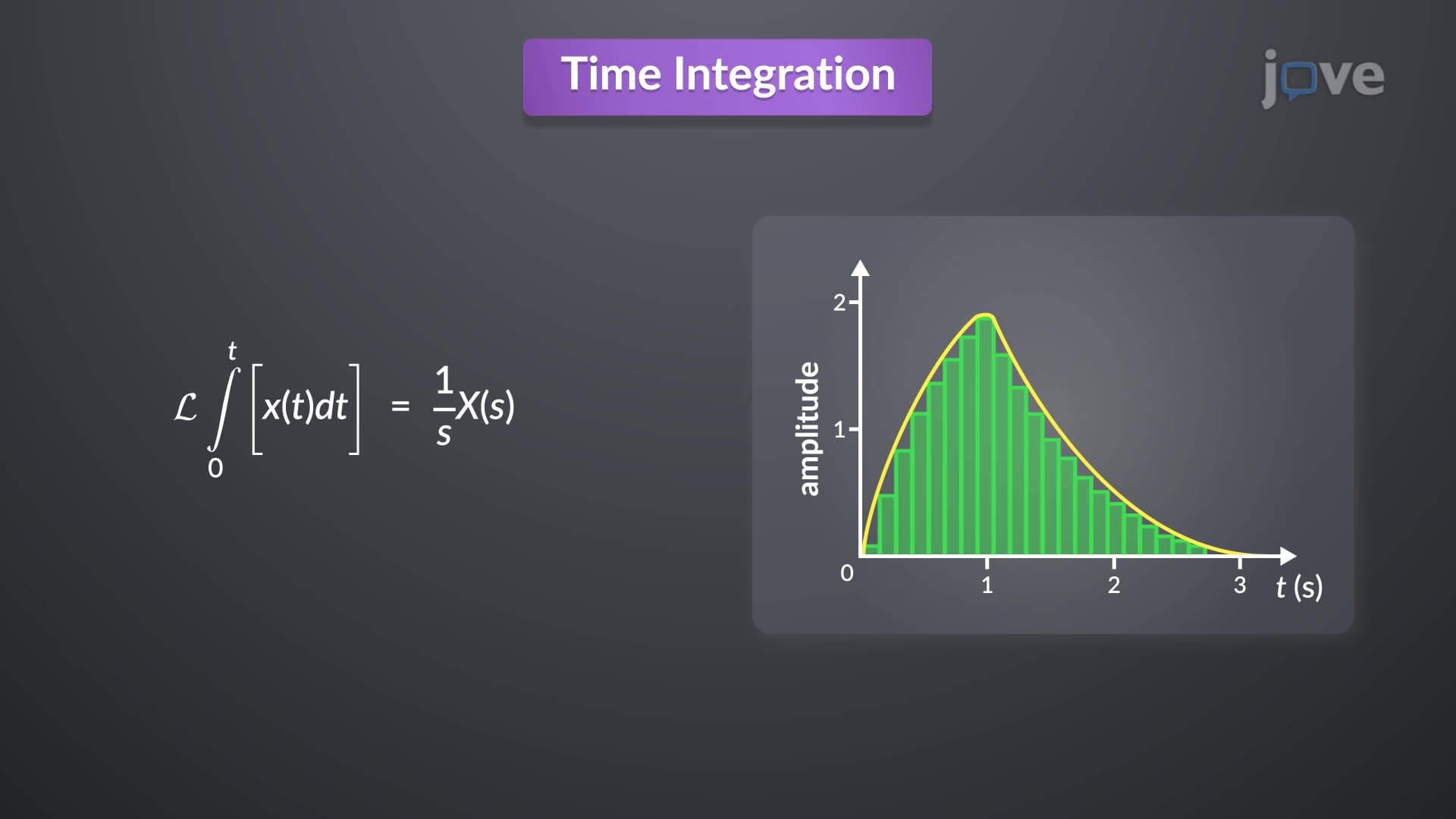
Did you know that pole and system stability analysis determines whether your smartphone's audio processing will produce clear sound or chaotic noise? The pole and system stability concept is fundamental to understanding how control systems behave over time. Engineers at Boeing use these principles when designing aircraft autopilot systems to ensure stable flight patterns. Properties of Laplace Transform II Explained provides the mathematical foundation for predicting system behavior. Watch the full video on JoVE Coach to master this concept with expert-led visuals and step-by-step explanations.

• Understand how Properties of Laplace Transform II Explained relate to pole locations and their impact on system stability
• Identify the relationship between pole positions in the s-plane and corresponding time-domain system responses
• Analyze how time differentiation properties affect pole-zero configurations in Laplace transforms
• Compare stable versus unstable system behaviors using pole and system stability criteria
• Evaluate system performance through convolution operations and their frequency domain representations
• Apply integration properties to determine long-term system behavior and steady-state responses
• Recognize periodic system patterns and their corresponding pole arrangements in complex analysis
• Explore real-world applications where pole and system stability determines design success

Understanding Properties of Laplace Transform II Explained

The pole and system stability concept forms the cornerstone of modern control theory and signal processing. A pole represents a frequency at which a system's response becomes theoretically infinite, while system stability determines whether small disturbances will grow or decay over time. This pole and system stability definition becomes critical when analyzing everything from car cruise control systems to NASA's spacecraft navigation.

Mathematical Foundation and Pole Analysis

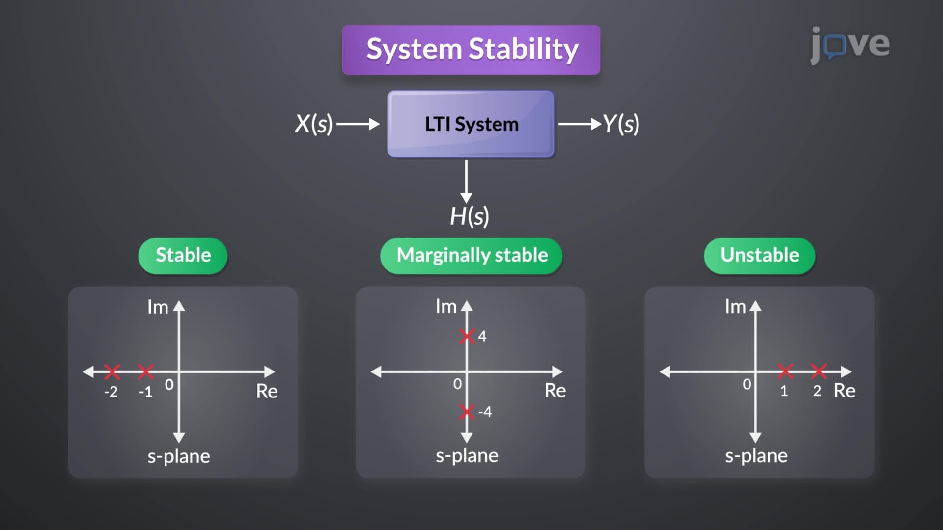
When examining pole and system stability in detail, we focus on the location of poles in the complex s-plane. Poles located in the left half-plane (negative real parts) indicate stable systems, while right half-plane poles signal instability. The pole and system stability overview reveals that poles on the imaginary axis create marginally stable systems that oscillate indefinitely.

Consider a second-order system with transfer function H(s) = K / (s² + 2ζωₙs + ωₙ²). The poles occur at s = -ζωₙ ± ωₙ√(ζ² - 1). For a damped oscillator like a car's suspension system, when ζ > 0, the poles have negative real parts, ensuring the vehicle returns to equilibrium after hitting a bump.

Time-Domain Properties and System Behavior

The pole and system basics extend to understanding how Laplace transform properties manifest in real systems. Time differentiation property shows that d/dt[f(t)] ↔ sF(s) - f(0), which directly relates to system dynamics. When Ford engineers design electric vehicle motor controllers, they use this property to predict acceleration responses.

Convolution in the time domain becomes multiplication in the frequency domain: f₁(t) * f₂(t) ↔ F₁(s)F₂(s). This principle underlies digital audio processing in streaming services like Spotify, where multiple audio signals combine to create final output.

Real-World Applications and Exam Relevance

Understanding the pole and system stability concept proves essential for AP Physics, college-level differential equations courses, and engineering programs. Students encounter these concepts in MCAT physics sections and advanced placement calculus exams. The pole and system stability study guide approach emphasizes practical problem-solving techniques used in industry.

Major applications include: power grid stability analysis (preventing blackouts like the 2003 Northeast blackout), aircraft flight control systems (ensuring safe autopilot operation), and medical device design (maintaining precise insulin pump delivery rates). Each application requires careful pole placement to guarantee stable, predictable system behavior under varying operating conditions.