Loading subject page…

- Physics
- Motion in Two or Three Dimensions
- Average and Instantaneous Velocity Vectors
Micro-course: Motion in Two or Three Dimensions
154,200 views
Learn key concepts and earn your certificate.

Average and Instantaneous Velocity Vectors

00:00
01:12
Video Summary: Average and Instantaneous Velocity Vectors Explained
Ever wonder why NASA engineers track spacecraft trajectories using velocity vectors rather than simple speed measurements? Average and instantaneous velocity vectors reveal both the magnitude and direction of motion in space, making them essential for everything from launching satellites to designing roller coasters at Six Flags. While average velocity describes motion over a time interval, instantaneous velocity captures the exact motion at a single moment-like photographing a baseball mid-flight during a Yankees game. Watch the full video on JoVE Coach to master this concept with expert-led visuals and step-by-step explanations.
- Understand how average and instantaneous velocity vectors differ in their mathematical definitions and physical interpretations
- Identify the relationship between displacement vectors and average velocity in two and three-dimensional coordinate systems
- Analyze how instantaneous velocity emerges as the mathematical limit when time intervals approach zero
- Compare velocity vector components in 2D versus 3D motion using unit vector notation
- Evaluate the geometric significance of instantaneous velocity vectors being tangent to the motion path
- Apply derivative calculus to find velocity components from position functions in multiple dimensions
- Recognize how velocity vector magnitude relates to an object's speed at any given instant
- Explore real-world applications where vector analysis is crucial for motion prediction and control
Understanding Average And Instantaneous Velocity Vectors
The distinction between average and instantaneous velocity vectors forms a cornerstone of kinematics that students encounter throughout physics education, from AP Physics courses to college-level mechanics. While scalar velocity only tells us "how fast," velocity vectors reveal both speed and direction-critical information for engineers designing everything from Tesla autopilot systems to SpaceX rocket trajectories.
Average Velocity: Motion Over Time Intervals
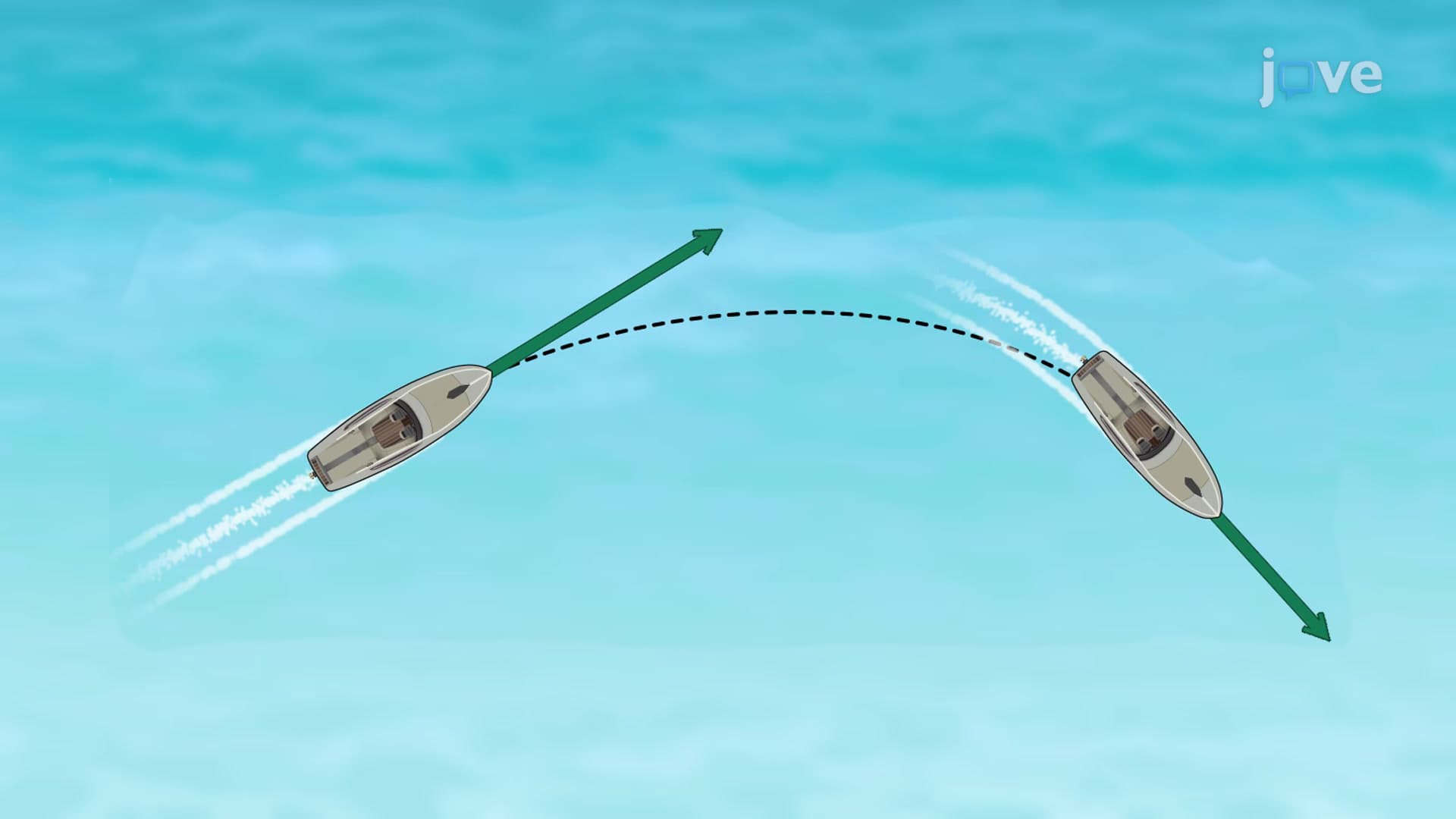
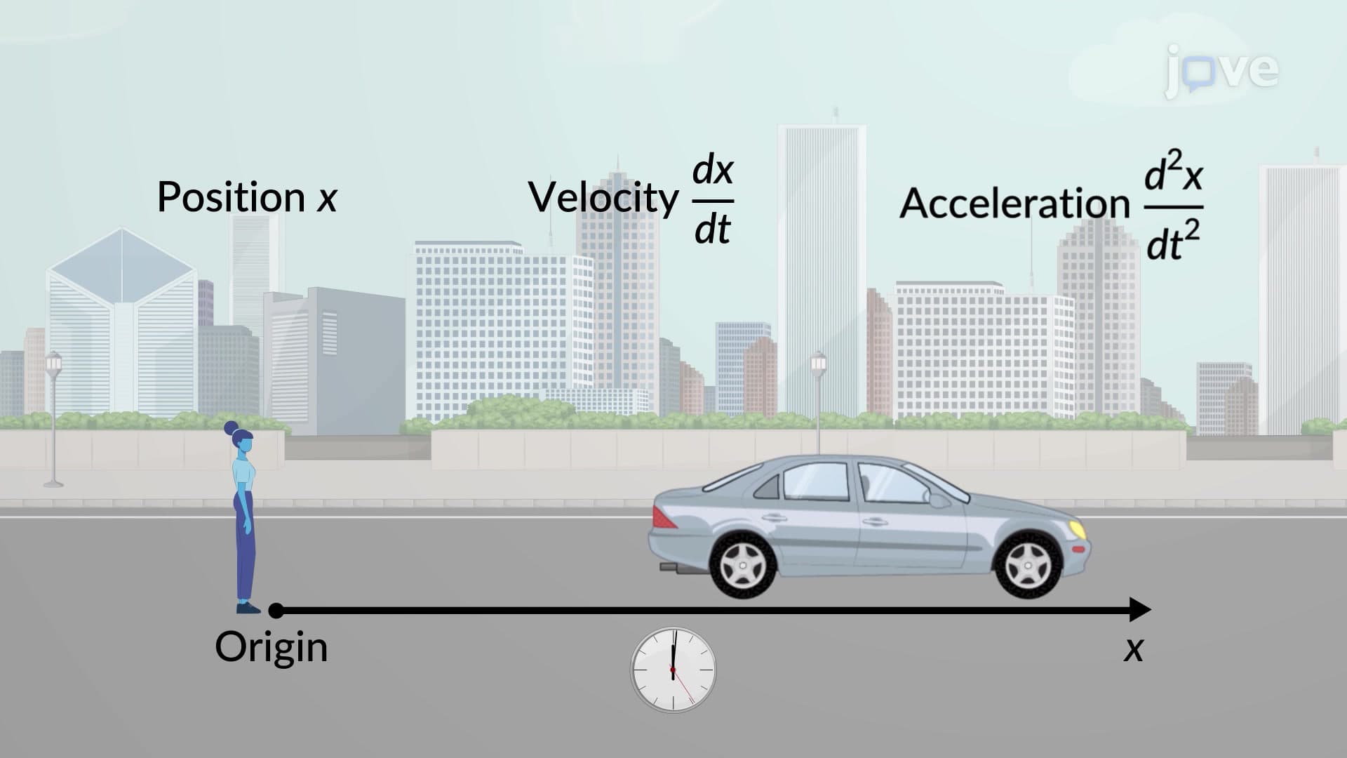
Average velocity represents the overall change in position divided by the elapsed time period. Mathematically, this appears as v(avg) = Δr/Δt, where Δr represents the displacement vector and Δt represents the time interval. Unlike average speed, which considers total distance traveled, average velocity focuses solely on the straight-line displacement from start to finish.
Consider a delivery drone flying from a Amazon warehouse in Seattle to a customer's home. Even if the drone follows a complex flight path around buildings and trees, its average velocity vector points directly from warehouse to destination, with magnitude determined by straight-line distance divided by total flight time. This concept proves essential for AP Physics 1 exam problems involving projectile motion and circular motion scenarios.
Instantaneous Velocity: Capturing Motion at a Single Moment
Instantaneous velocity emerges when we examine motion at infinitesimally small time intervals. As Δt approaches zero, the average velocity approaches the instantaneous velocity through calculus limits: v(instant) = dr/dt. This derivative relationship connects position functions directly to velocity vectors, making it a frequent topic on college calculus-based physics exams.
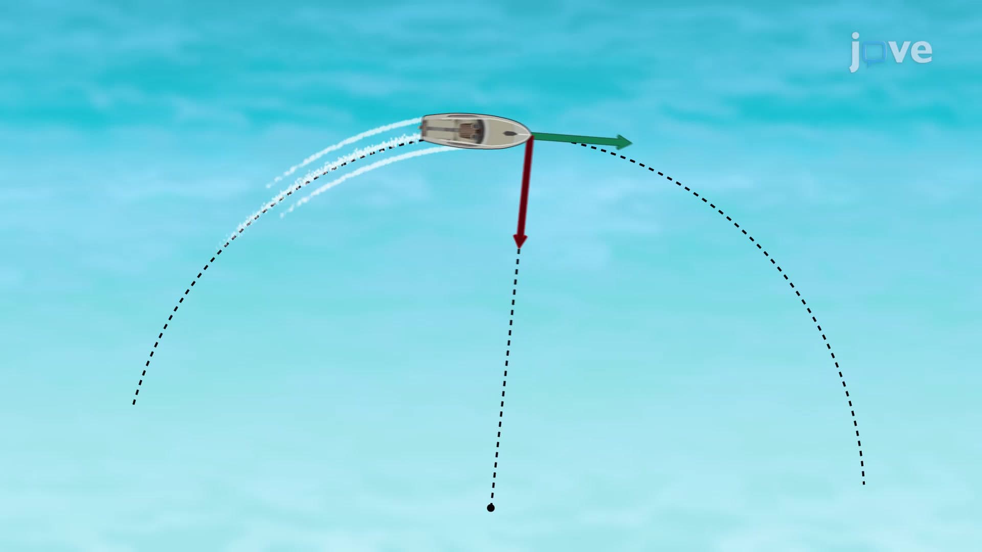
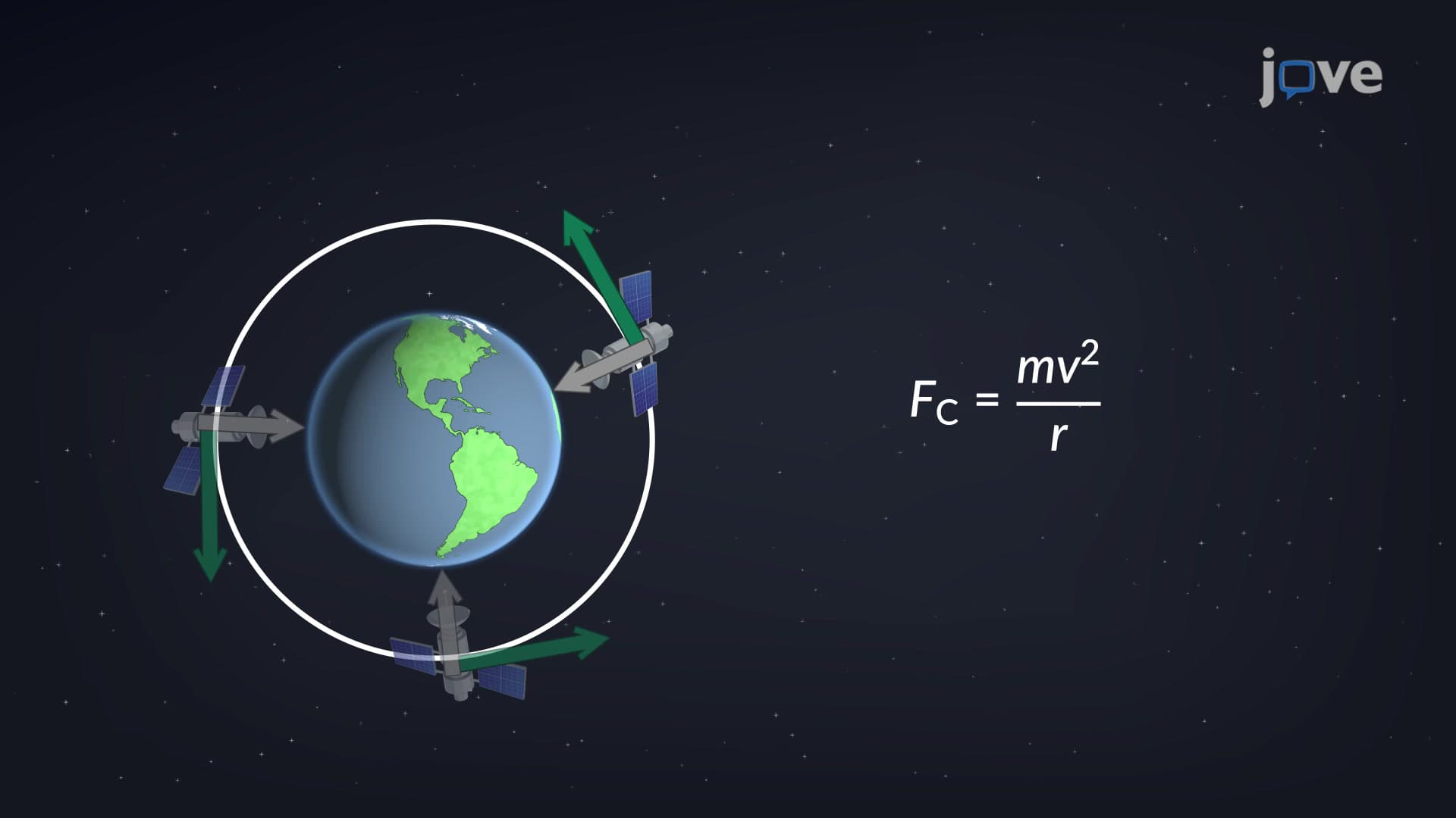
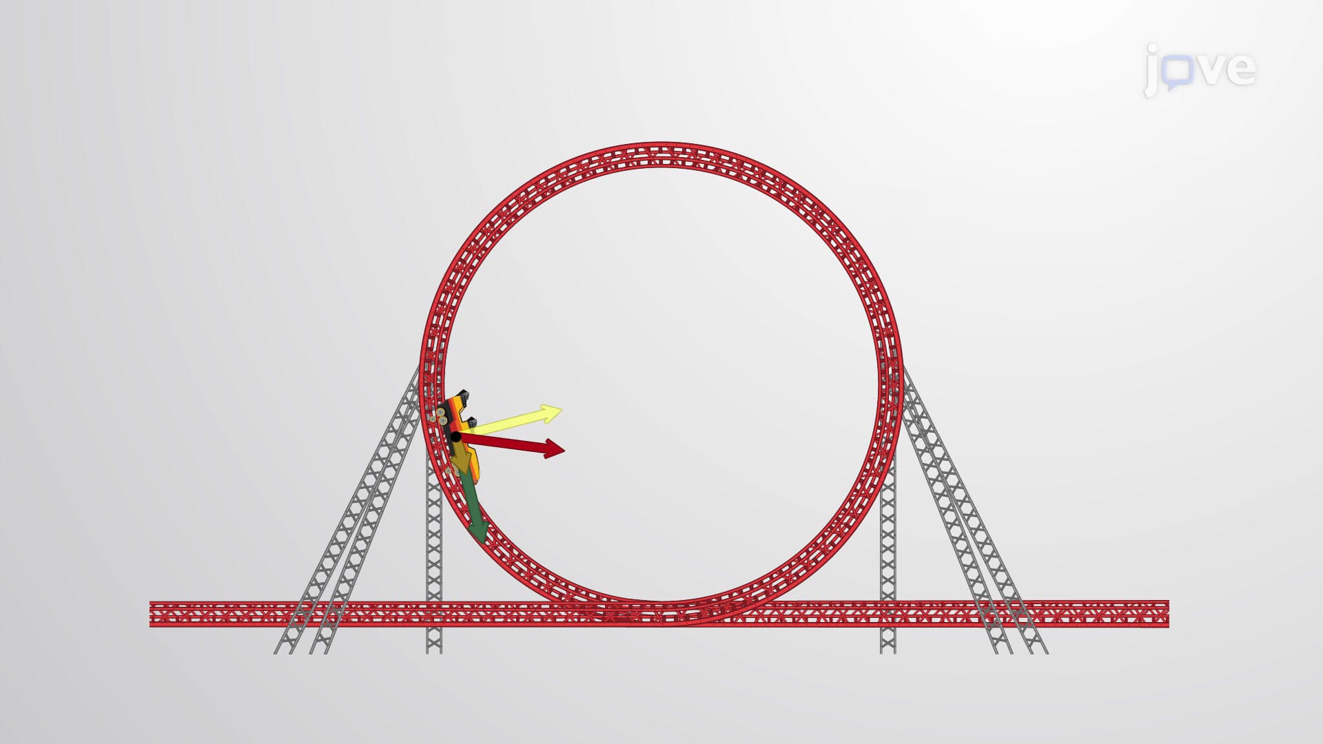
The geometric interpretation reveals that instantaneous velocity vectors always align tangentially to the motion path. Picture a NASCAR driver navigating Daytona International Speedway-at any specific moment, their velocity vector points along the track's tangent line at that exact position, not toward the track's center.
Multi-Dimensional Vector Components
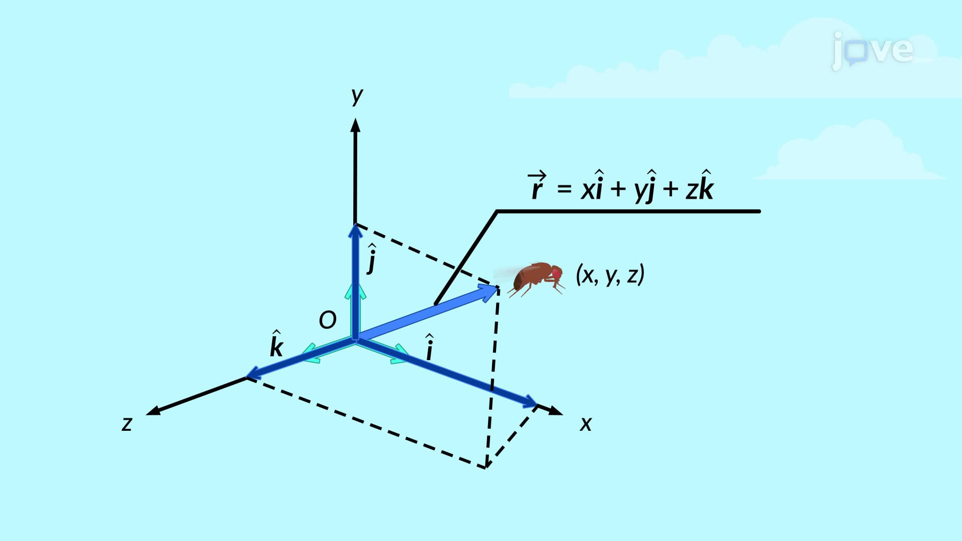
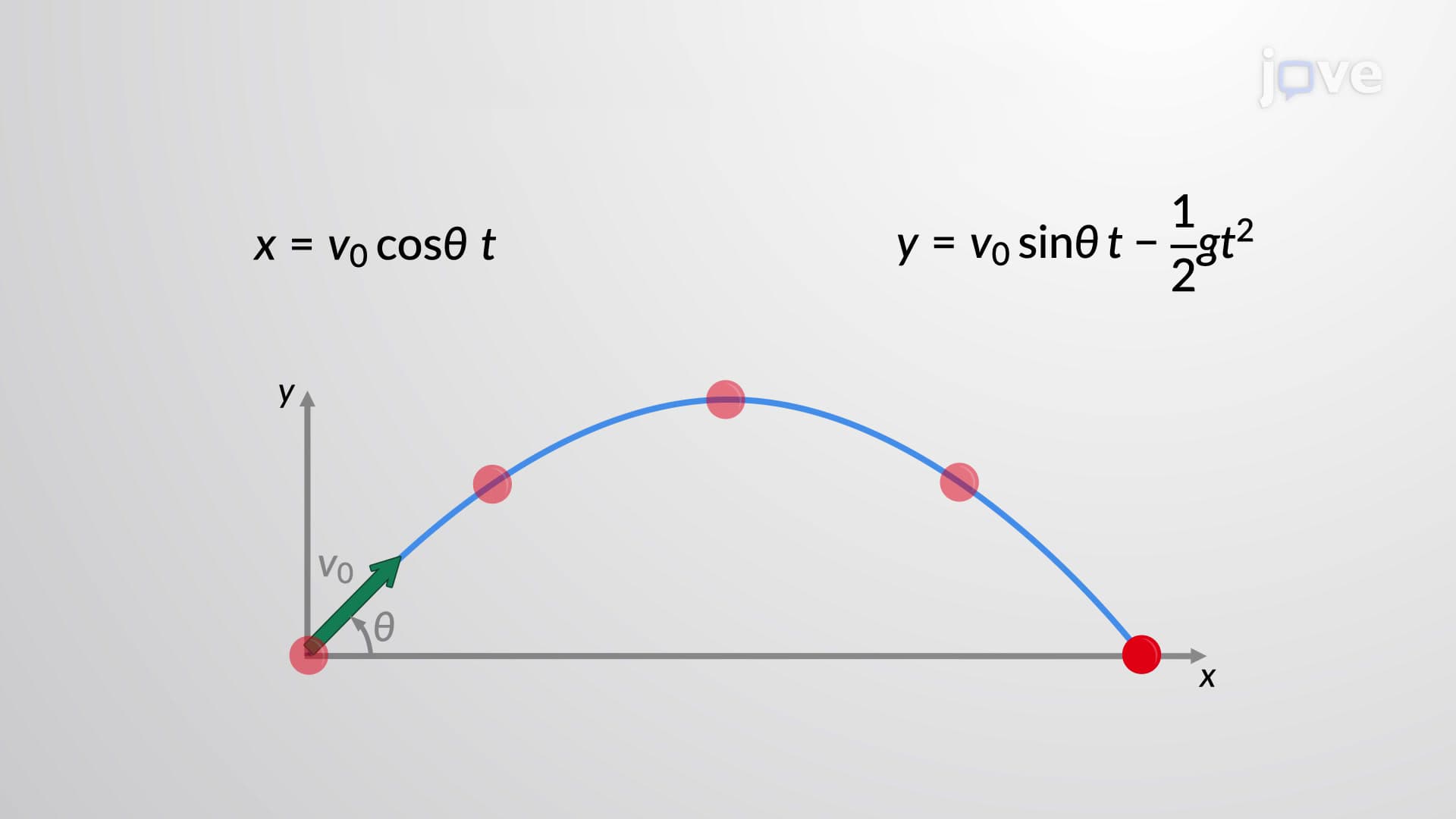
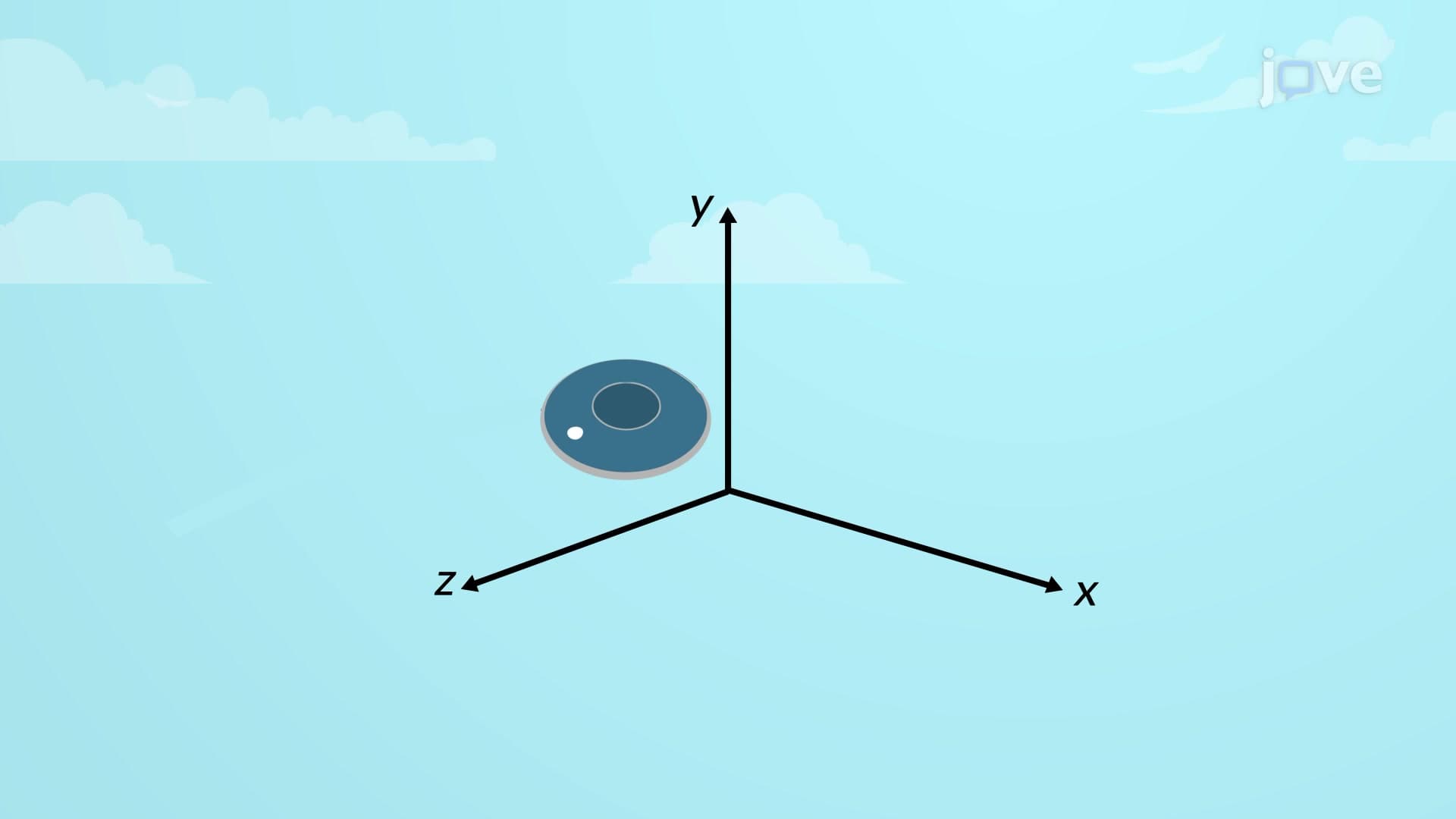
In two-dimensional motion, velocity vectors split into perpendicular components: v = vx(i) + vy(j), where i and j represent unit vectors along x and y axes respectively. Three-dimensional motion adds the z-component: v = vx(i) + vy(j) + vz(k). Each component equals the time derivative of its corresponding position coordinate, allowing students to analyze complex motions by examining simpler one-dimensional components separately.
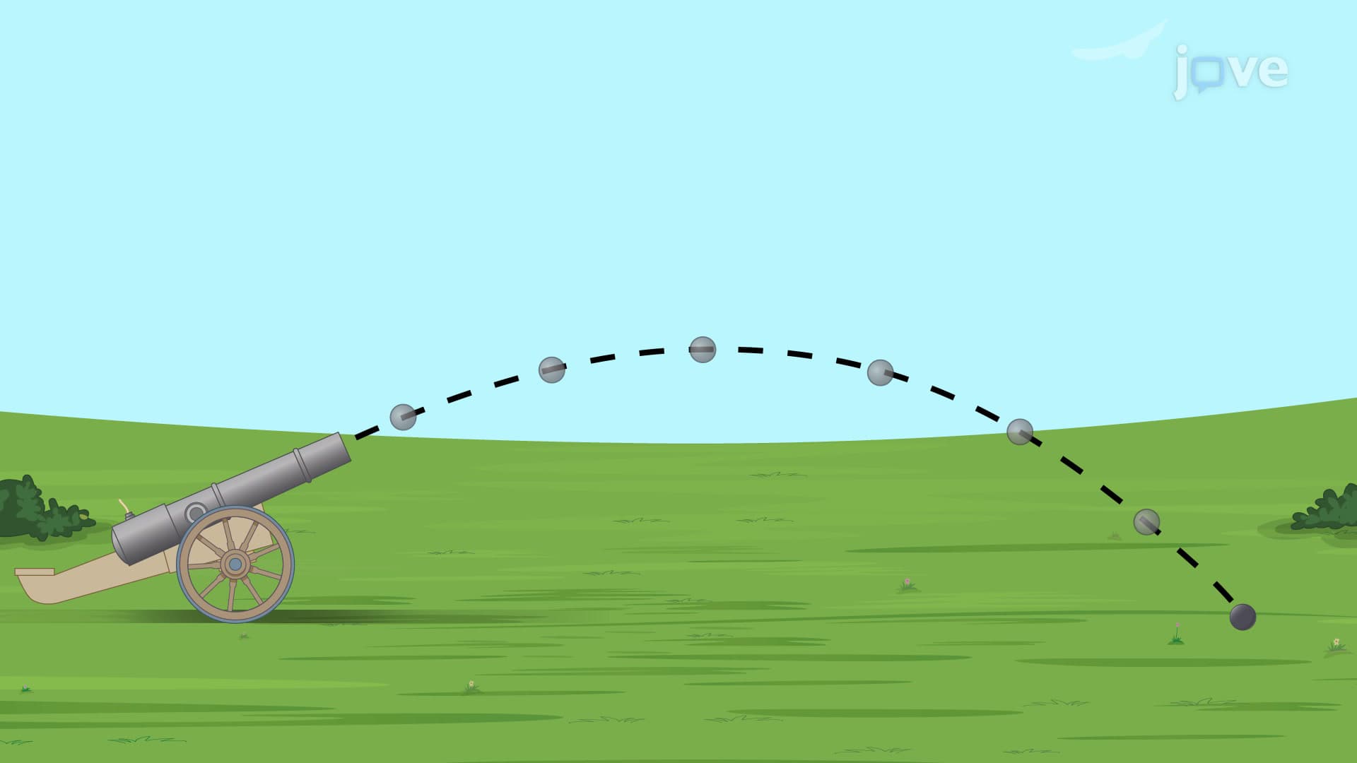
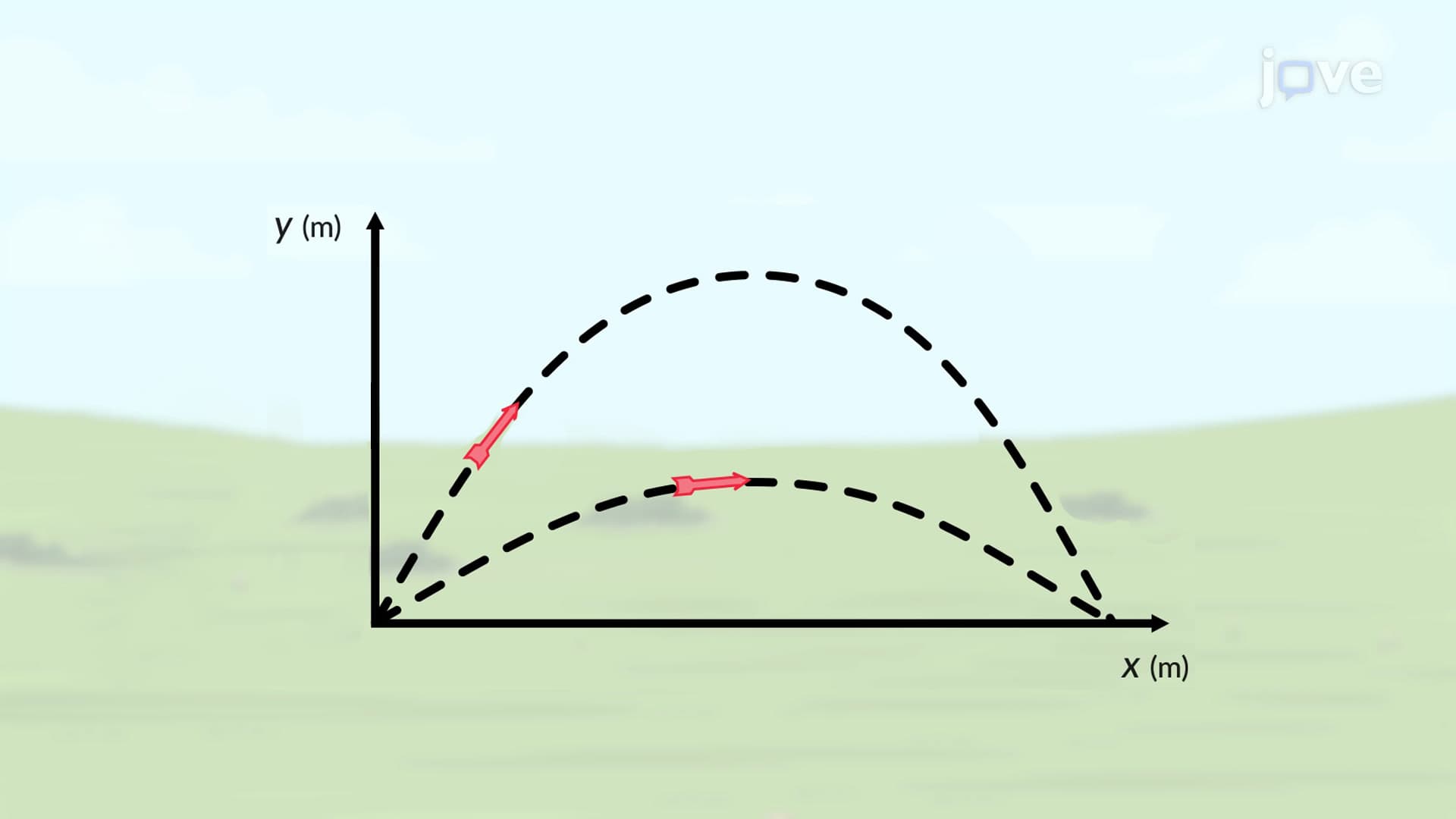
This component analysis proves invaluable for MCAT physics sections, where students must analyze projectile motion problems involving objects launched at angles-think football field goals or basketball free throws at Duke University's Cameron Indoor Stadium.
Frequently Asked Questions
Average velocity vectors describe motion over a finite time period using total displacement divided by elapsed time, while instantaneous velocity vectors capture the exact motion at a single moment through calculus derivatives. Average velocity smooths out motion variations, whereas instantaneous velocity reveals moment-by-moment changes in both speed and direction.
AP Physics 1 and C exams frequently test velocity vectors through projectile motion, circular motion, and relative motion scenarios. Students must calculate components, find resultant vectors, and interpret graphs showing position versus time relationships. Expect questions involving objects moving in parabolic paths, like launched projectiles or satellite orbits.
You need solid understanding of derivatives, limits, and vector notation for college-level physics courses. Instantaneous velocity involves taking derivatives of position functions with respect to time: v = dr/dt. Many universities require Calculus I as a prerequisite or corequisite for physics courses covering these topics.
NASA engineers use velocity vectors to calculate spacecraft trajectories, orbital mechanics, and landing sequences for missions like the Mars Perseverance rover. Mission control continuously tracks both magnitude and direction of spacecraft velocity to execute precise maneuvers, dock with the International Space Station, and land rovers on planetary surfaces with pinpoint accuracy.
Mathematically, instantaneous velocity represents the derivative dr/dt, which geometrically corresponds to the slope of the position curve at that exact point. Since tangent lines represent instantaneous rates of change on curves, the velocity vector naturally aligns tangentially to show the direction of motion at that precise moment.
Practice drawing vector diagrams, breaking complex motions into components, and connecting graphical representations to mathematical equations. Focus on projectile motion problems, work through AP Physics practice tests, and master the relationship between position, velocity, and acceleration graphs. Regular problem-solving builds intuition for vector analysis.
Yes, you can grasp the fundamental concepts using basic algebra and trigonometry, though calculus enhances understanding significantly. High school physics courses introduce velocity vectors through geometric approaches and component analysis, making the concepts accessible before students encounter formal derivative calculations in college courses.
Build on velocity vector knowledge by exploring acceleration vectors, force analysis using Newton's laws, and energy methods in mechanics. Advanced topics include rotational motion, oscillations, and wave mechanics. These concepts form the foundation for upper-level courses in electromagnetism, thermodynamics, and modern physics.
Related Micro-courses
16 Concepts

10 Concepts
15 Concepts