Loading video…


 7 Concepts
 1.7K views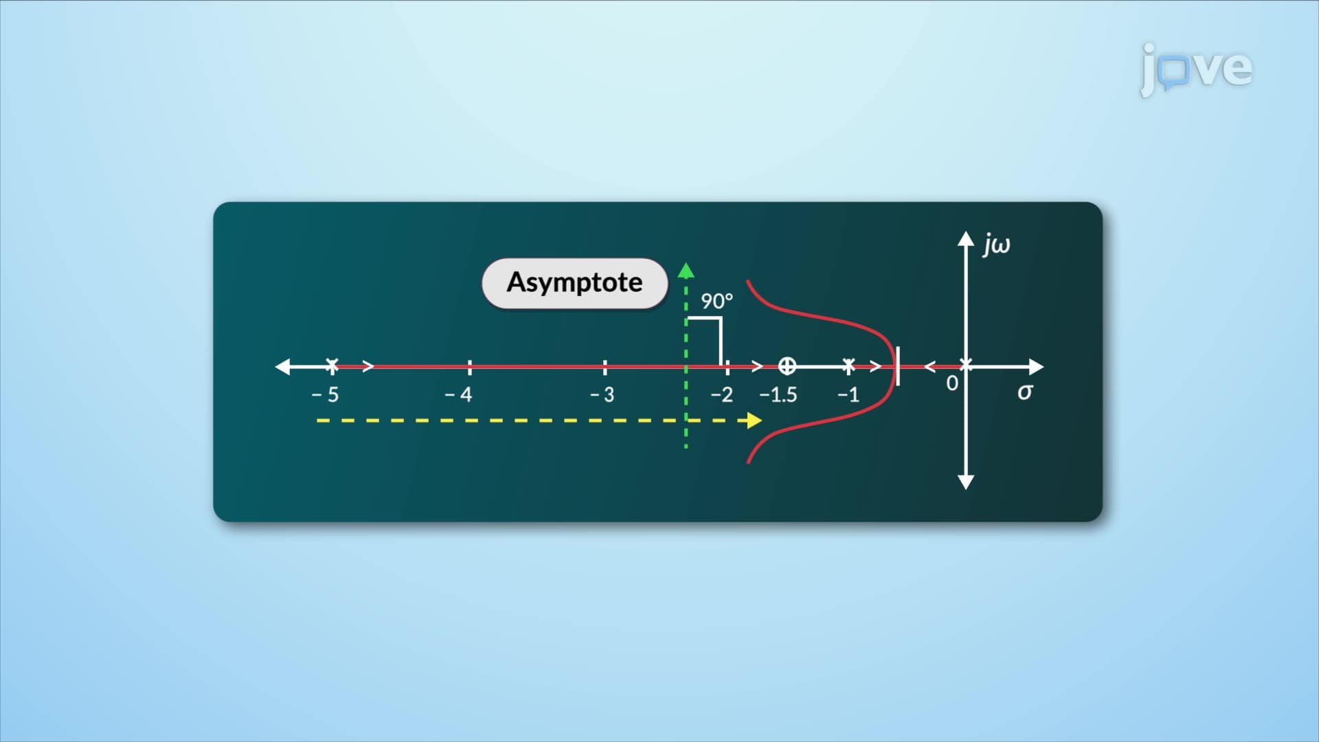

Video Summary: What Is Construction of Root Locus
Ever wonder how NASA engineers ensure rocket guidance systems remain stable during launch? The secret lies in plotting and calibrating the root locus, a powerful graphical method that predicts how control systems behave as parameters change. Consider Boeing's autopilot systems: engineers use root locus construction to map exactly where system poles move as gain increases, ensuring aircraft maintain stable flight from takeoff to landing. Understanding the construction of root locus reveals the mathematical roadmap that transforms open-loop instability into closed-loop precision. Watch the full video on JoVE Coach to master this concept with expert-led visuals and step-by-step explanations.
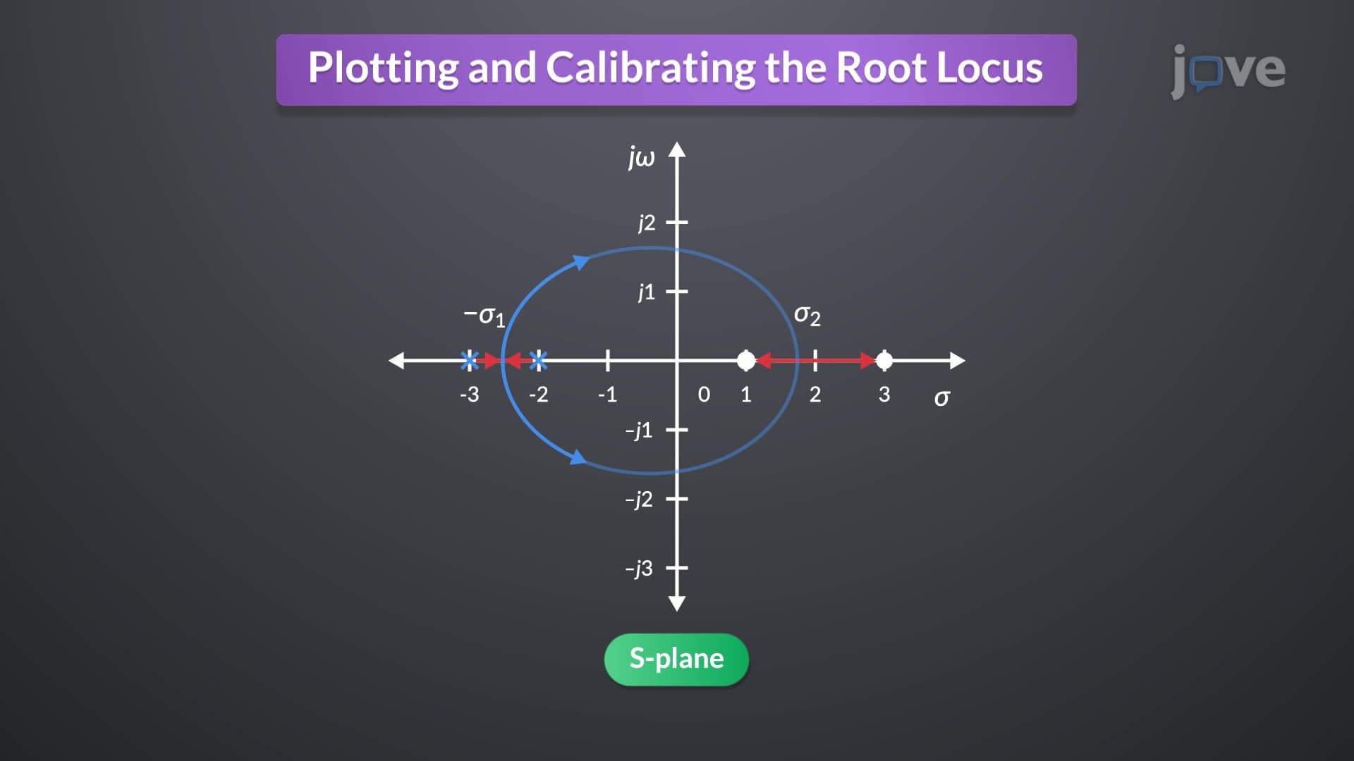
The construction of root locus represents one of control theory's most elegant graphical techniques, providing engineers with a visual roadmap of system behavior. At its core, root locus construction maps the journey of closed-loop poles as system gain K increases from zero to infinity. This mathematical framework proves invaluable for students preparing for AP Physics C exams or engineering coursework, where understanding system stability determines success.
Root locus construction follows predictable geometric patterns that simplify complex analysis. The most fundamental rule establishes symmetry about the real axis, if a complex pole exists at location s = a + jb, its conjugate must exist at s = a - jb. This symmetry reflects the physical reality that real systems with real coefficients produce complex poles in conjugate pairs.
The real-axis rule provides another crucial construction guideline: root locus exists on real-axis segments where the total number of finite open-loop poles and zeros to the right sums to an odd number. For example, consider a system with poles at s = -1, -3, -5 and a zero at s = -2. The root locus exists between s = -2 and s = -3, and also between s = -5 and negative infinity, because these segments satisfy the odd-sum criterion.
As gain approaches infinity, root locus branches approach straight-line asymptotes. The number of asymptotes equals the difference between the number of finite poles and finite zeros. These asymptotes intersect the real axis at the centroid, calculated using: σ = (sum of pole locations - sum of zero locations)/(number of poles - number of zeros).
The asymptote angles follow the formula: θ = (2k + 1)180°/(n - m), where n represents poles, m represents zeros, and k = 0, 1, 2, ... This mathematical precision enables engineers at companies like Lockheed Martin to predict exactly how aircraft control systems will behave under varying conditions.
Root locus construction directly impacts real-world engineering decisions. Tesla's autopilot systems rely on these principles to maintain vehicle stability across varying speeds and road conditions. Similarly, medical device manufacturers use root locus analysis to ensure ventilators respond appropriately to patient breathing patterns without oscillation or instability.
Students encountering this material in college controls courses or preparing for the Fundamentals of Engineering exam will find root locus construction bridges theoretical mathematics with practical system design, making it an essential tool for aspiring engineers across aerospace, automotive, and biomedical industries.
Related Micro-courses