Graphing Antiderivatives

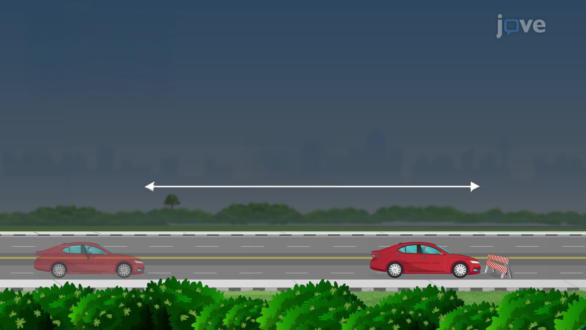
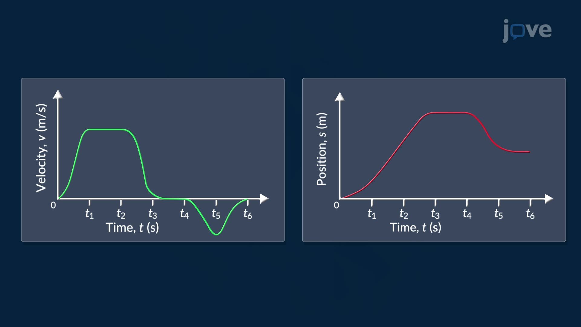
Ever wonder how a car's speedometer reading connects to its physical position on the highway? Graphing antiderivatives basics reveals exactly that link — turning a velocity curve into a position graph using calculus logic. A classic US highway driving scenario illustrates how positive, negative, and zero velocity values shape whether a position function rises, falls, or curves. Watch the full video on JoVE Coach to master this concept with expert-led visuals and step-by-step explanations.

• Understand what graphing antiderivatives means and how the shape of a derivative graph directly determines the behavior of its antiderivative function
• Identify intervals where the antiderivative is increasing, decreasing, or constant based on the sign of the original function's values
• Analyze concavity of the antiderivative graph by observing whether the given function (the derivative) is itself increasing or decreasing over each interval
• Recognize inflection points on the antiderivative graph as locations where the derivative function changes from increasing to decreasing or vice versa
• Apply maximum and minimum value reasoning to determine where the antiderivative reaches a peak or valley — specifically where the derivative equals zero and changes sign
• Compare straight-line segments on an antiderivative graph to intervals where the derivative is constant and nonzero, reinforcing the relationship between slope and linearity
• Evaluate real-world motion scenarios — such as a vehicle's speed profile over time — to construct a qualitative position graph without computing an explicit formula
• Explore connections between graphing antiderivatives and broader calculus topics like curve sketching, the Mean Value Theorem, and optimization problems

Graphing Antiderivatives Explained: Turning Derivative Graphs into Function Graphs

Graphing antiderivatives is one of the most visually intuitive skills in calculus — and one of the most tested. Rather than computing a formula, you interpret the graph of a derivative and reconstruct the behavior of the original function. This skill sits at the heart of AP Calculus AB and BC, college-level Calculus I courses across US universities, and even standardized assessments like the AP exam's free-response section.

The Sign of the Derivative Controls Rising and Falling

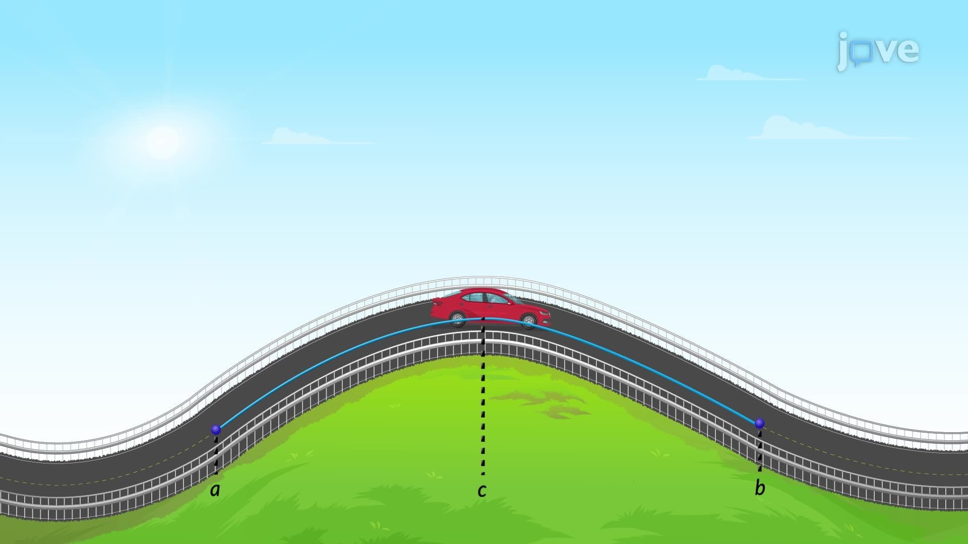
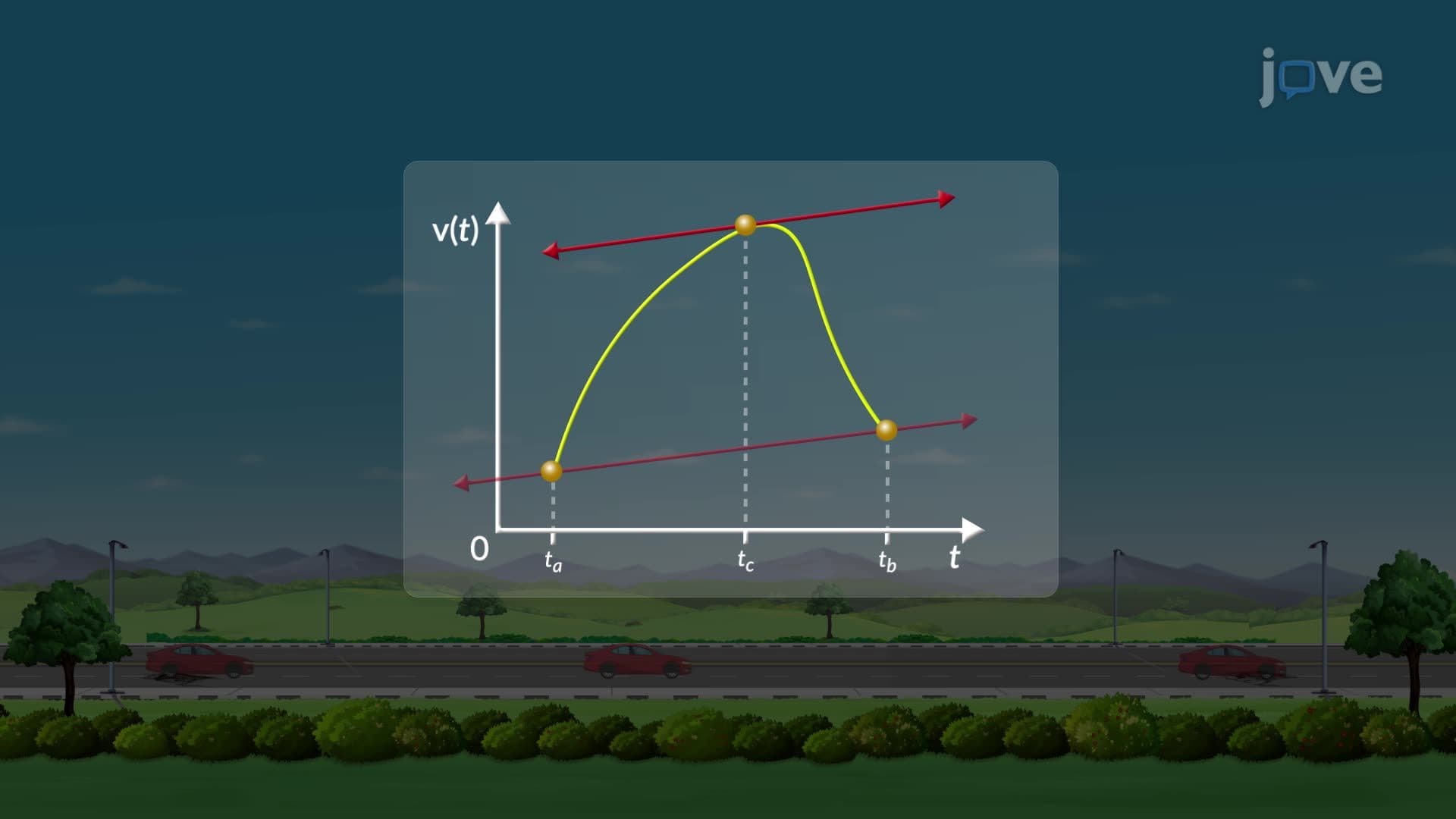
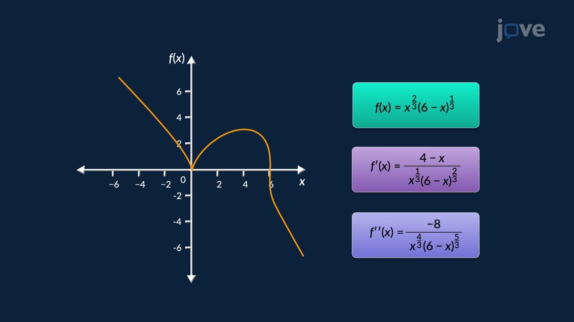
The most fundamental rule in graphing antiderivatives is this: wherever the derivative (let's call it f'(x)) is positive, the antiderivative F(x) is increasing. Wherever f'(x) is negative, F(x) is decreasing. When f'(x) equals zero, F(x) has a horizontal tangent — a potential maximum or minimum value. Think of a speedometer on an interstate highway in Texas: when the speedometer reads above zero, the car is moving forward and its position is increasing. When the reading drops to zero at a rest stop, position temporarily holds steady.

This sign analysis is the same logic used in curve sketching and directly connects to finding maximum and minimum values on any function — a core skill in optimization problems throughout Calculus I and II.

Concavity and Inflection Points: Reading the Derivative's Own Slope

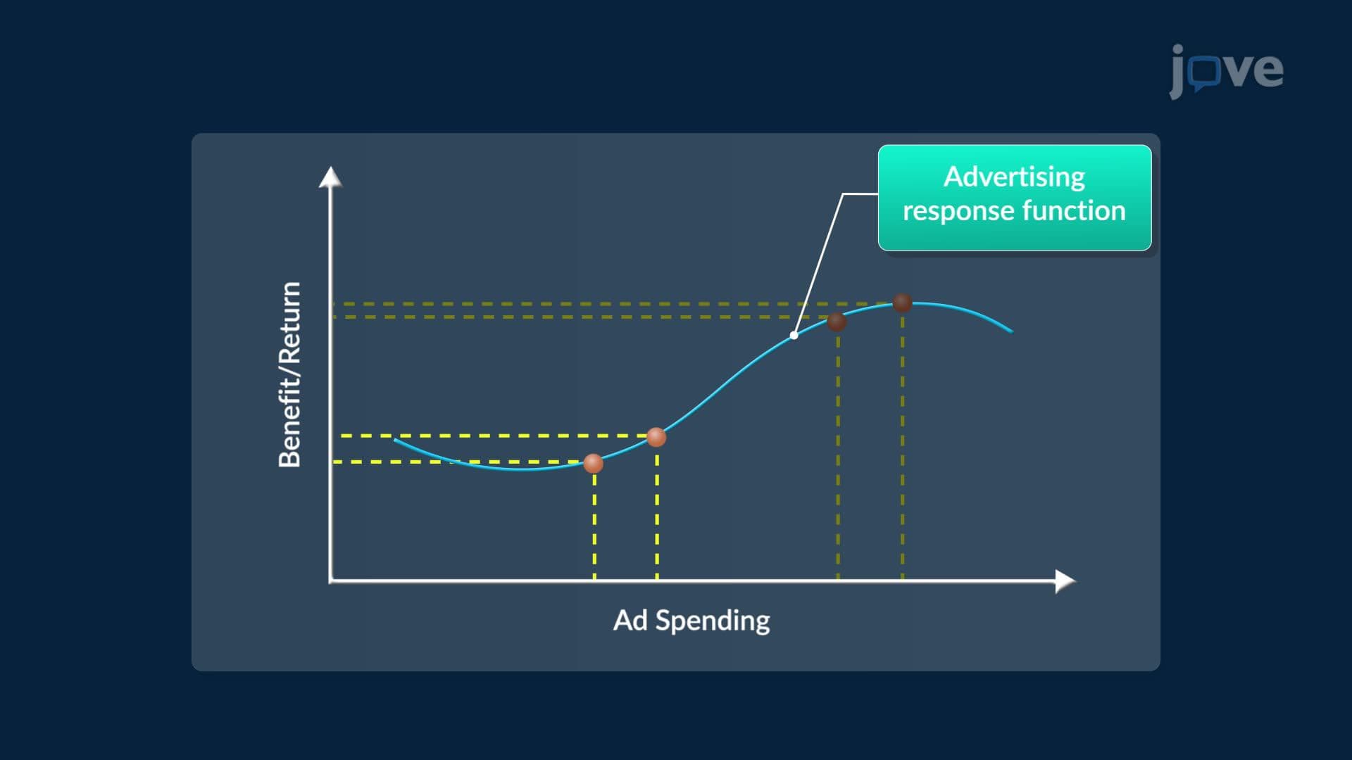
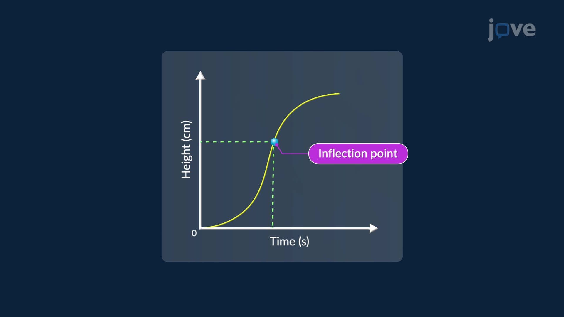
Concavity of the antiderivative depends on whether the derivative function is increasing or decreasing — not just positive or negative. If f'(x) is increasing over an interval (its values are climbing), then F(x) is concave up on that interval, bending like a bowl. If f'(x) is decreasing, F(x) is concave down, arching like a hill. An inflection point on F(x) occurs precisely where f'(x) switches from increasing to decreasing, or the reverse.

This mirrors the second derivative test used in optimization problems and curve sketching: when the second derivative (which is the derivative of f'(x)) changes sign, concavity switches. On AP Calculus exams, questions routinely ask students to identify inflection points from a given derivative graph — making this a high-priority skill.

Straight Lines, Constant Slopes, and the Mean Value Theorem Connection

When the derivative graph is flat and constant — say, a horizontal line at a positive value — the antiderivative produces a perfectly straight, upward-sloping line segment. This is because a constant derivative means the rate of change is uniform, exactly what the Mean Value Theorem guarantees must exist somewhere on a smooth curve. US college professors frequently use this relationship in midterm problems, asking students to match derivative graph segments to antiderivative graph shapes.

Why This Skill Matters Beyond the Classroom

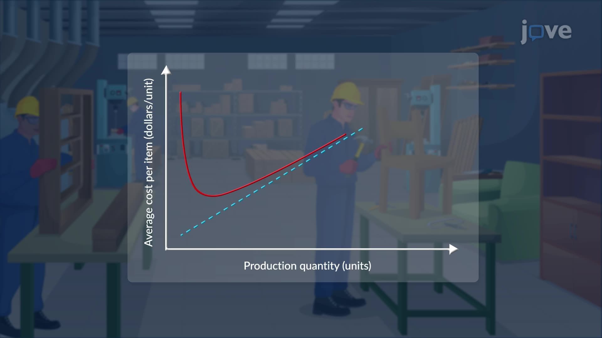
Graphing antiderivatives appears in physics courses at US universities when reconstructing displacement from a velocity-time graph, in economics when recovering a total cost function from a marginal cost graph, and in engineering when analyzing motion profiles for robotics or vehicle dynamics. On the AP Calculus AB exam, this concept typically appears in both multiple-choice and free-response questions, often disguised as related rates or motion analysis scenarios. Mastering the visual logic — sign implies direction, slope of derivative implies concavity — allows students to answer these questions confidently without needing an explicit algebraic antiderivative formula.