Savings, Consumption and Investment

Savings economics forms the foundation of macroeconomic theory, examining how households and businesses allocate income between current consumption and future needs. This comprehensive course explores the intricate relationship between savings consumption and investment, covering essential concepts like the marginal propensity to consume, consumption functions, and macroeconomic savings theory. Students will master Keynesian models and analyze real-world applications through JoVE Coach's systematic approach to understanding economic equilibrium.

• Understand the fundamental definitions of consumption, savings, and investment in macroeconomic contexts
• Learn to calculate and interpret the marginal propensity to consume and save in economic models
• Identify the differences between private and public savings and their impact on national economies
• Explore consumption functions and break-even points in household spending decisions
• Analyze the Permanent Income Hypothesis and Life-Cycle Hypothesis theories
• Apply savings-investment equilibrium models to predict economic outcomes
• Understand how interest rates influence planned investment decisions
• Learn to construct and interpret planned aggregate expenditure schedules
• Analyze the relationship between wealth, income expectations, and consumption patterns
• Apply economic theories to real-world scenarios involving fiscal policy and household finance

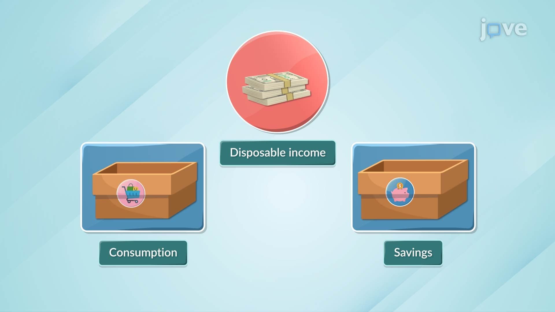
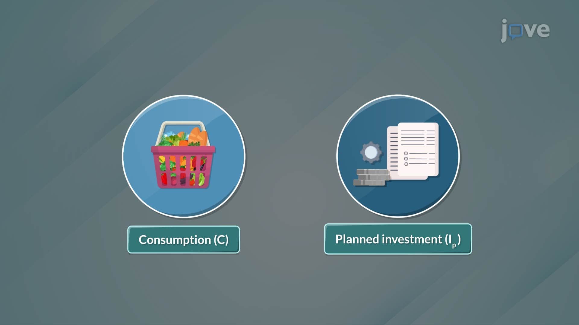
1. Fundamental Economic Definitions and Classifications Consumption represents household spending on goods and services for immediate satisfaction, such as a Denver family purchasing groceries, clothing, and entertainment. Savings constitute the portion of disposable income not consumed, like a Seattle tech worker setting aside $500 monthly from their $4,000 salary. Investment involves business spending on capital goods that enhance future production capacity, exemplified by a Texas manufacturing company purchasing new machinery. These three components form the backbone of macroeconomic analysis, determining how economies allocate resources between present needs and future growth opportunities.

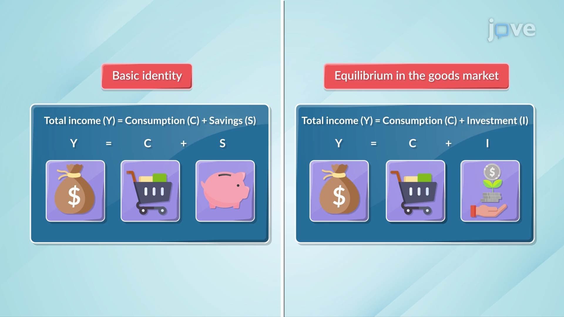
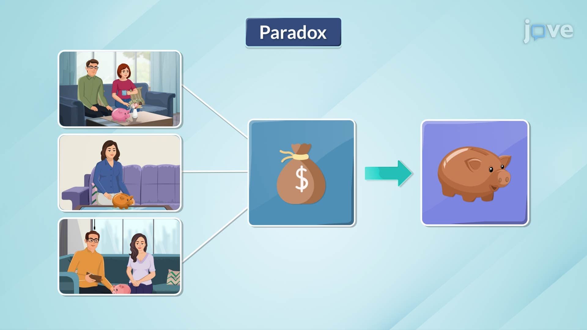
2. Private vs. Public Savings and National Accounting Private savings (S = Y - T - C) represent household income remaining after taxes and consumption, while public savings (T - G) reflect government fiscal balance between tax revenue and spending. When California households save $200 billion annually and the state government runs a $50 billion surplus, total savings equal $250 billion. In closed economies, national savings must equal total investment, establishing the fundamental macroeconomic identity that drives economic equilibrium. Understanding this relationship helps predict how fiscal policy changes affect overall economic activity and resource allocation patterns.

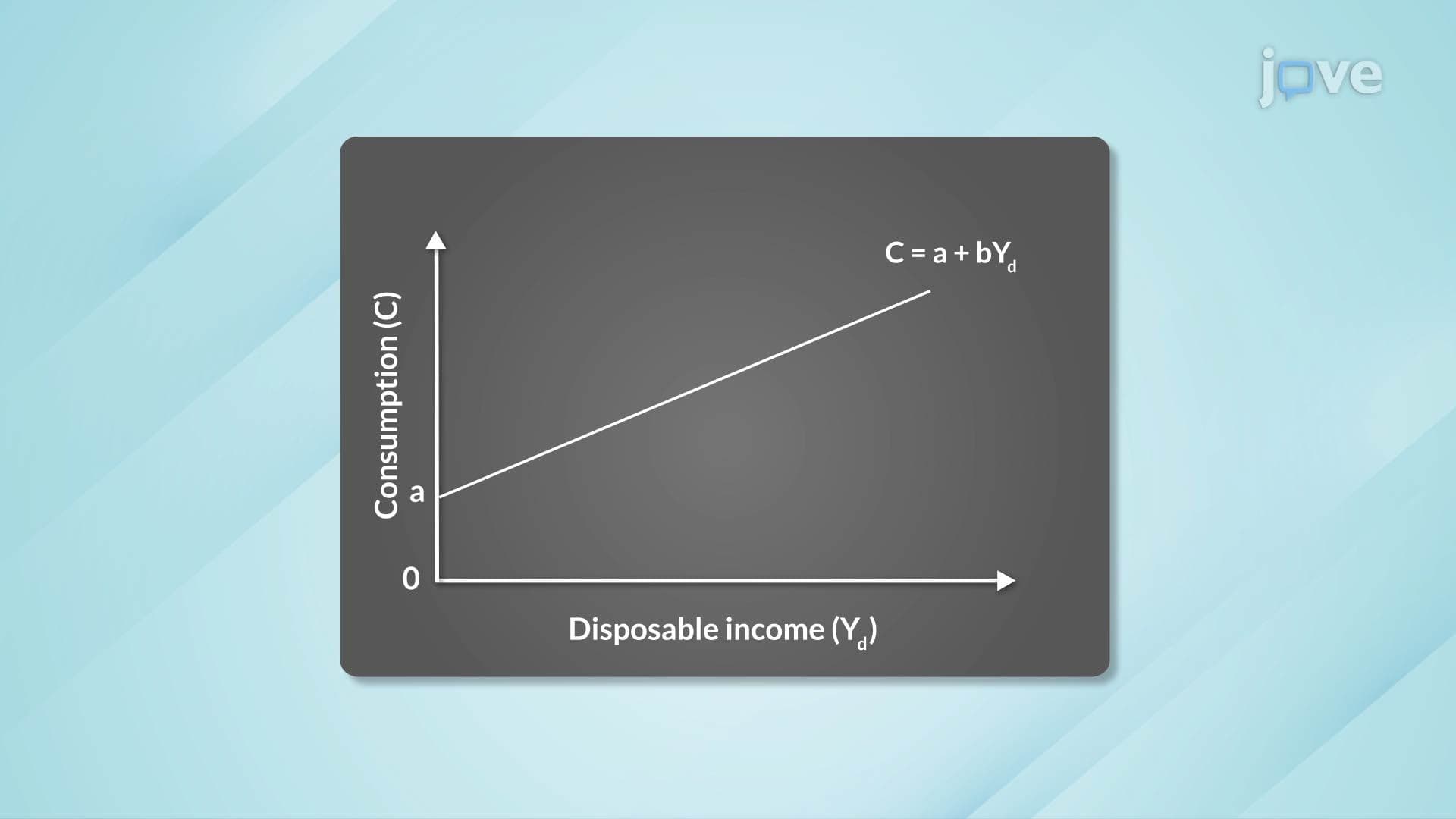
3. The Consumption Function and Marginal Propensity to Consume The consumption function (C = a + bYd) describes how household spending responds to income changes, where 'a' represents autonomous consumption and 'b' measures the marginal propensity to consume. If a Chicago family has autonomous consumption of $1,000 monthly and an MPC of 0.75, they spend $750 of every additional $1,000 earned. This relationship enables economists to predict how tax cuts or income changes affect aggregate demand. The consumption function's slope determines the investment multiplier effect, crucial for understanding fiscal policy impacts on economic growth and stability.

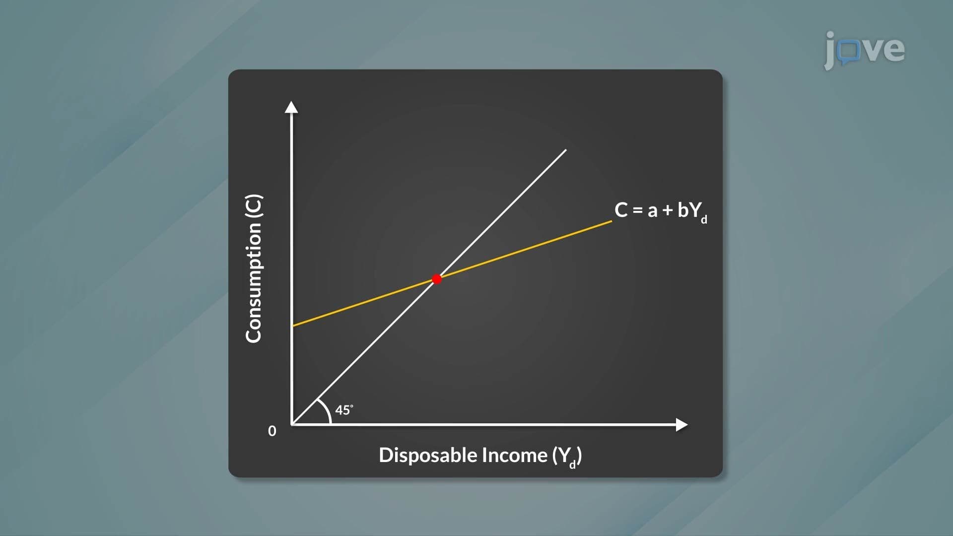
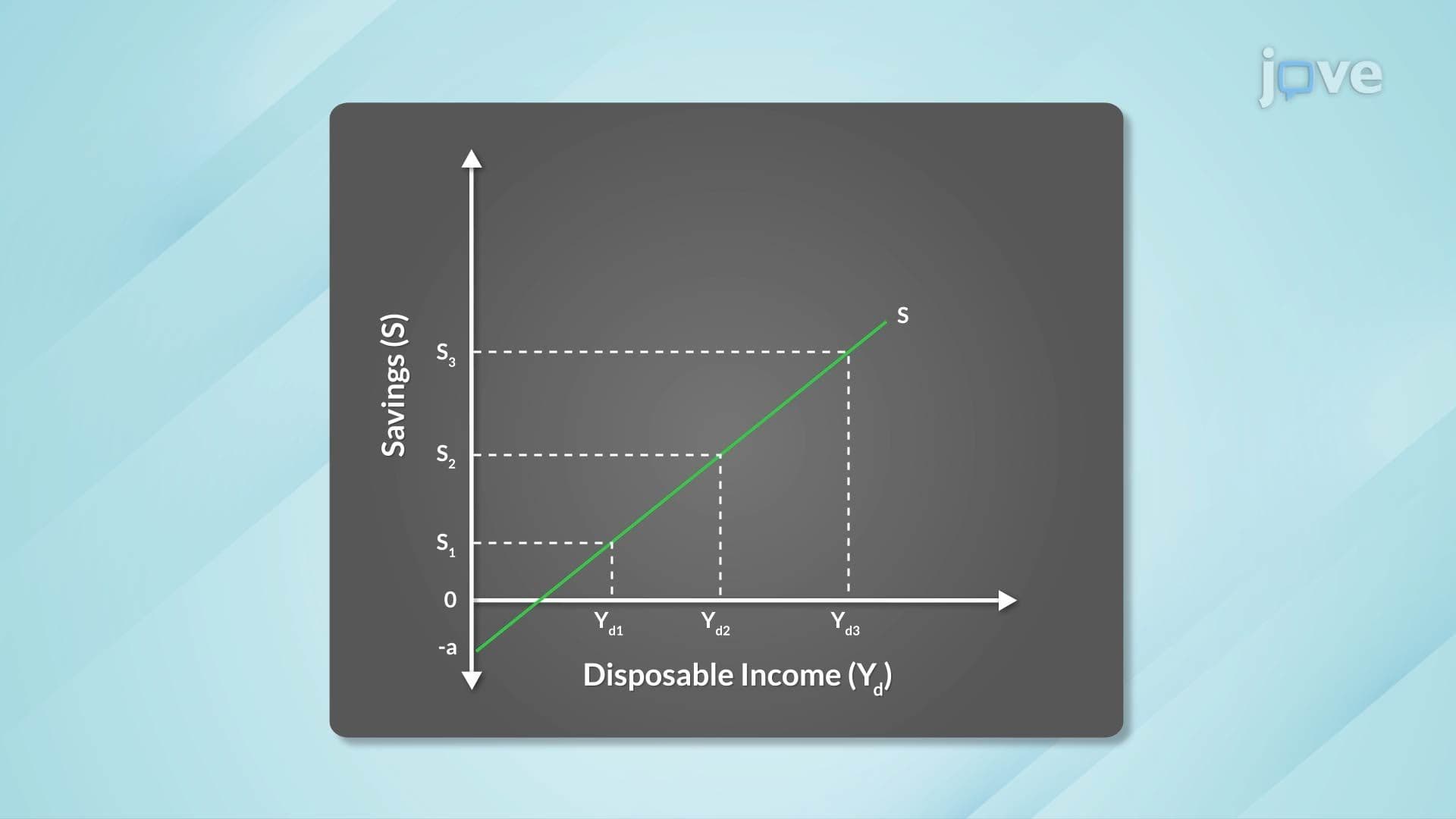
4. Savings Function and Break-Even Analysis The savings function (S = Yd - C) illustrates how much households save at different income levels, typically showing negative savings at low incomes due to borrowing or asset depletion. The break-even point occurs where consumption equals income (savings = zero), calculated as autonomous consumption divided by (1 - MPC). For example, with autonomous consumption of $2,000 and MPC of 0.8, break-even income equals $10,000. Below this point, households dissave by borrowing or using assets; above it, they accumulate savings for future needs, retirement, or emergencies.

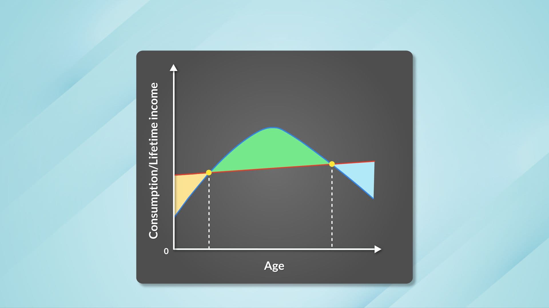
5. Advanced Consumption Theories: Permanent Income and Life-Cycle Hypotheses Milton Friedman's Permanent Income Hypothesis suggests consumers base spending on expected lifetime income rather than current earnings, explaining why lottery winners don't dramatically increase consumption immediately. The Life-Cycle Hypothesis predicts individuals borrow during early career years, save heavily during peak earning periods, and spend accumulated wealth during retirement. A typical American professional might borrow for education at 25, save aggressively from 40-60, then draw down savings after 65. These theories explain consumption smoothing behavior and help predict responses to temporary versus permanent income changes.

6. Investment Theory and Interest Rate Effects Planned investment depends inversely on real interest rates, as higher borrowing costs reduce profitable project opportunities. When the Federal Reserve raises rates from 2% to 5%, construction companies postpone building projects because financing costs exceed expected returns. Actual investment may differ from planned investment due to unexpected inventory changes - if Ford produces 100,000 vehicles but sells only 85,000, the 15,000 unsold cars represent unplanned investment. This distinction helps explain short-term economic fluctuations and adjustment mechanisms toward equilibrium through inventory changes and production adjustments.

7. Aggregate Expenditure and Macroeconomic Equilibrium Planned aggregate expenditure (AE = C + I) represents total intended spending in an economy, achieving equilibrium when it equals actual output. Using a 45-degree line diagram, equilibrium occurs where the aggregate expenditure curve intersects the output line. If planned spending exceeds output, unplanned inventory reductions signal firms to increase production; if output exceeds spending, inventory accumulation prompts production cuts. The savings-investment approach (S = I) provides an alternative equilibrium condition, demonstrating that economic balance requires matching society's desire to save with businesses' investment plans.