Solving Inequalities Graphically

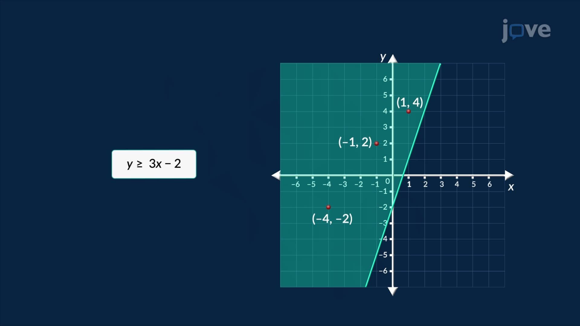
• Understand what is solving inequalities graphically and how visual methods reveal solution sets through coordinate plane analysis
• Identify the key steps: plotting functions, determining boundary lines, and shading appropriate regions based on inequality symbols
• Analyze intersection points between linear and quadratic functions to establish solution boundaries
• Compare different inequality types (greater than, less than, greater than or equal to) and their corresponding shaded regions
• Evaluate overlapping regions when solving systems of inequalities to find common solution sets
• Apply graphical inequality solving to real-world scenarios like budget analysis and constraint optimization
• Recognize when quadratic inequalities create parabolic boundaries versus linear inequalities forming straight-line boundaries
• Explore how graphical solutions connect to algebraic methods for comprehensive problem-solving approaches

Understanding Solving Inequalities Graphically: The Visual Approach

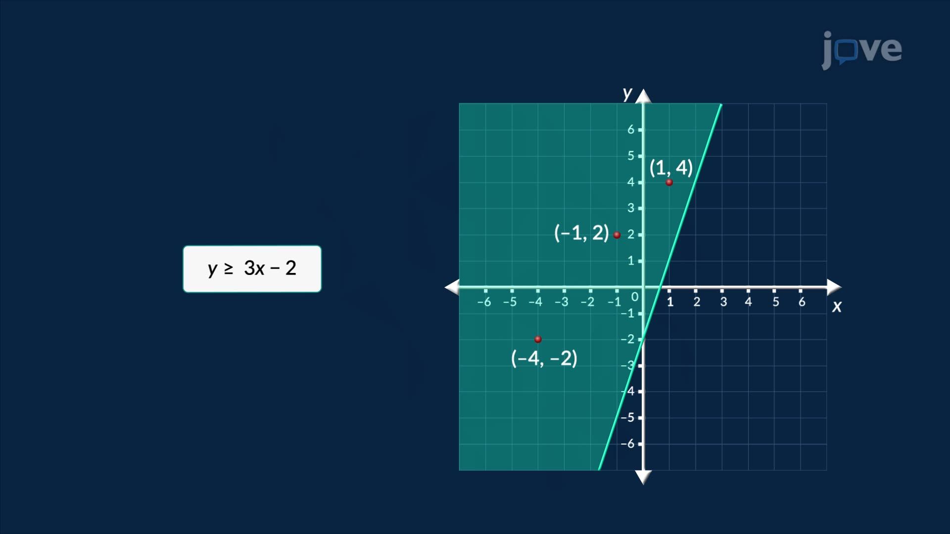
Solving inequalities graphically transforms mathematical relationships into visual representations that make solution sets immediately apparent. Unlike algebraic methods that require step-by-step manipulation, graphical approaches leverage the coordinate plane to show exactly where one expression exceeds, equals, or falls below another. This method proves particularly valuable for complex inequalities involving quadratic functions or systems of multiple constraints.

The Step-by-Step Graphical Process

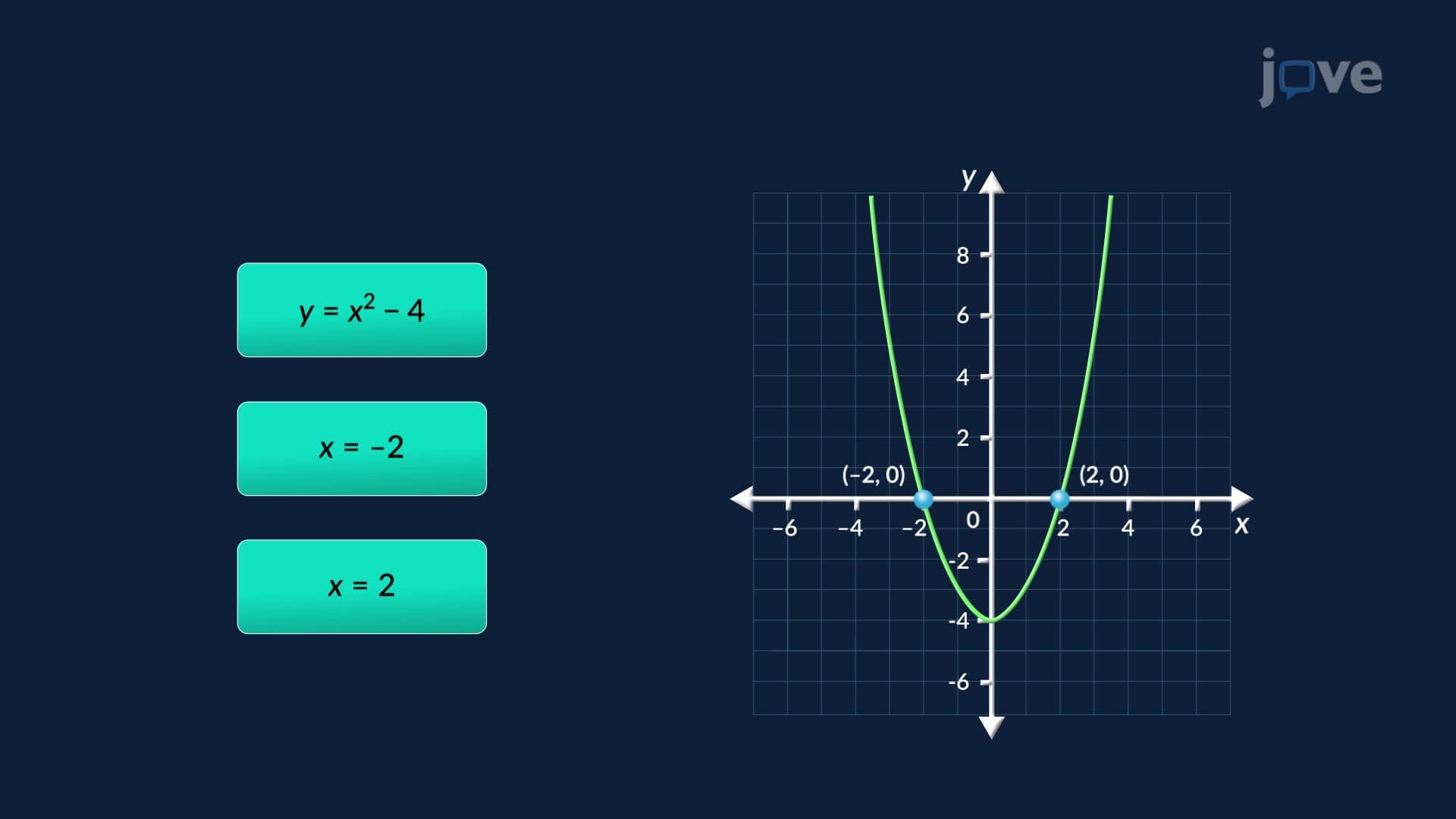
The graphical method begins by treating each side of an inequality as a separate function. For a quadratic inequality like x² - 2x - 3 ≥ 0, you first graph the parabola y = x² - 2x - 3. The x-intercepts occur where the parabola crosses the x-axis, marking critical boundary points. For inequalities involving "greater than or equal to" (≥), you shade the region where the parabola lies above or on the x-axis. Conversely, "less than or equal to" (≤) inequalities require shading where the function falls below or touches the x-axis.

When comparing two functions, such as a quadratic and linear inequality, both graphs appear on the same coordinate plane. Their intersection points become crucial boundary markers. Students taking the AP Calculus exam frequently encounter these mixed-function inequalities, where understanding the graphical relationship between different function types proves essential for success.

Systems of Inequalities and Overlapping Regions

Advanced applications involve multiple inequalities creating systems with overlapping solution regions. Consider a business scenario where a manufacturing company must satisfy both material cost constraints and production capacity limits. Each constraint creates its own boundary line, and the feasible solution exists only in the overlapping shaded region. This concept appears regularly on SAT Math Level 2 tests and college algebra midterms.

Real-World Applications in US Contexts

Financial institutions like Bank of America use graphical inequality solving for risk assessment models. Investment portfolios must satisfy multiple constraints simultaneously: minimum return requirements, maximum risk tolerance, and regulatory compliance limits. Each constraint creates a boundary on the investment space, and viable portfolios exist only in the intersection of all acceptable regions. Similarly, NASA engineers use these techniques for spacecraft trajectory planning, where fuel consumption and safety margins create multiple inequality constraints that must be satisfied simultaneously.