Short-run vs Long-run: Marginal Costs

• Understand how comparing short-run and long-run marginal cost curves reveals fundamental differences in production efficiency across time horizons
• Identify the key distinction between fixed inputs in short-run production versus variable inputs in long-run scenarios
• Analyze why short-run marginal cost curves intersect average total cost curves at minimum points
• Compare how long-run marginal cost curves are constructed using intersection points of short-run and long-run average cost curves
• Evaluate the relationship between long-run average total cost and long-run marginal cost curves during rising and falling phases
• Apply marginal cost concepts to real business decisions involving production scaling and capacity planning
• Recognize the mathematical relationship where marginal cost curves lie below average cost curves when averages are falling
• Explore how firms achieve greater efficiency in long-run production through optimal input combinations

Understanding Short-Run and Long-Run Marginal Cost Curves

The distinction between short-run and long-run marginal costs represents one of microeconomics' most practical concepts. In the short run, at least one production input remains fixed-typically capital like machinery, buildings, or equipment. This constraint forces firms to add variable inputs (usually labor) to existing fixed resources, creating the characteristic U-shaped short-run marginal cost curve that students encounter on AP Economics exams.

Short-Run Marginal Cost Dynamics

Short-run marginal cost (MC SR) measures the additional cost of producing one more unit when some inputs cannot be adjusted. Consider Tesla's Fremont factory: in the short run, the facility size and major assembly equipment are fixed. To increase Model 3 production, Tesla must add more workers, materials, and energy to existing production lines. Initially, additional workers increase efficiency through specialization, lowering marginal costs. However, as production pushes against capacity constraints, workers become less productive due to overcrowding and equipment limitations, causing marginal costs to rise sharply.

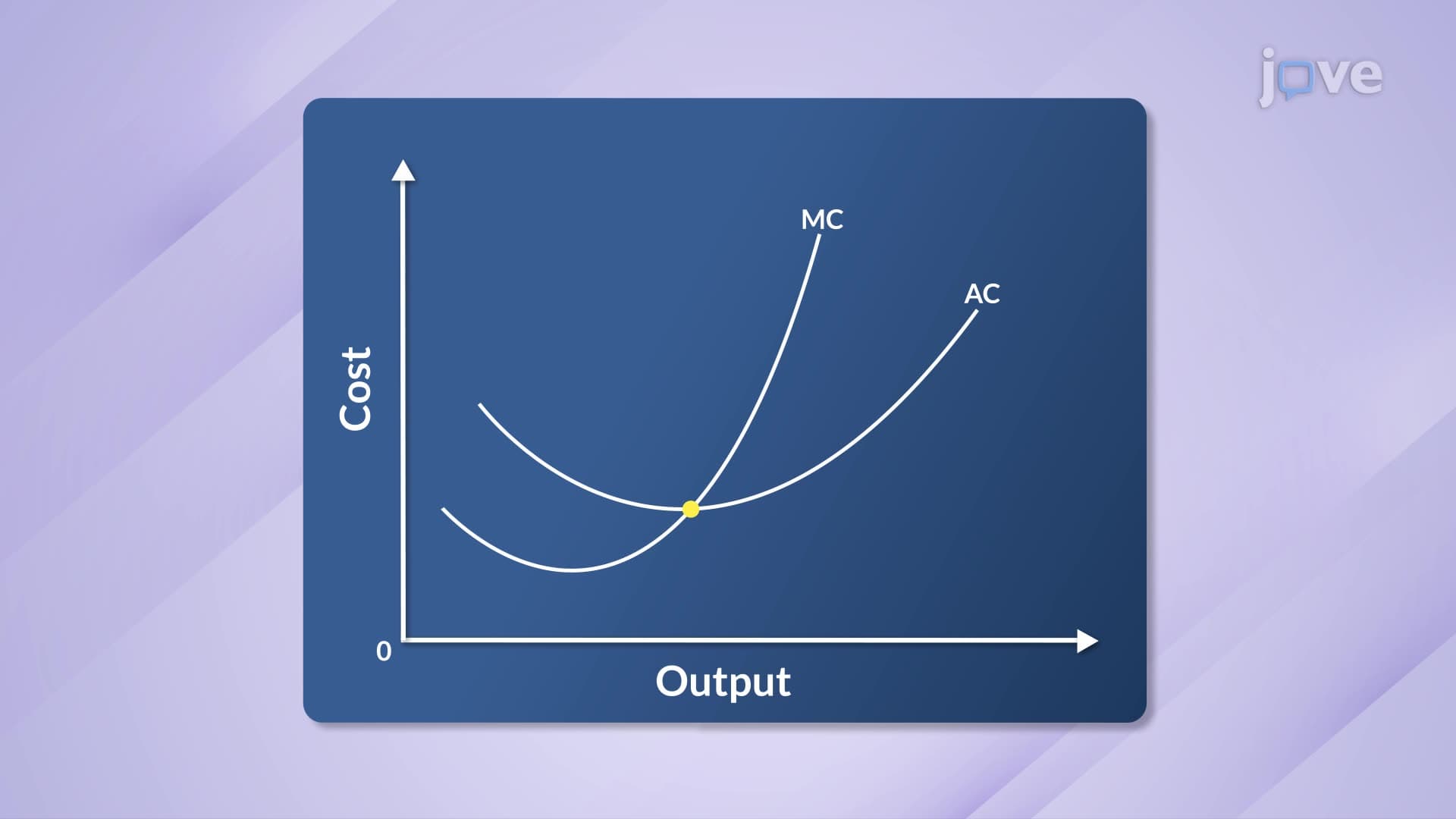
This creates the mathematical relationship where short-run marginal cost curves intersect their corresponding average total cost curves at the minimum point-a critical concept for college microeconomics courses and standardized tests.

Long-Run Marginal Cost Construction

Long-run marginal cost (MC LR) emerges when all inputs become variable, allowing firms complete flexibility in production decisions. The construction of this curve involves identifying where short-run average total cost curves intersect the long-run average total cost envelope curve. At these intersection points, firms operate at optimal efficiency for their chosen scale.

The long-run marginal cost curve connects corresponding quantity points from different short-run marginal cost curves, creating a smoother, more efficient cost structure. This explains why companies like Walmart can achieve lower per-unit costs by optimizing everything from store locations to supply chain networks over extended periods.

Practical Applications and Exam Implications

Understanding these relationships proves essential for AP Economics students and college economics majors. The key insight-that long-run marginal cost lies below long-run average total cost when averages are falling, and above when averages are rising-appears frequently on multiple-choice exams and essay questions. Both curves intersect at the minimum point of long-run average total cost, representing the most efficient production scale.