Loading video…


 9 Concepts
 5K views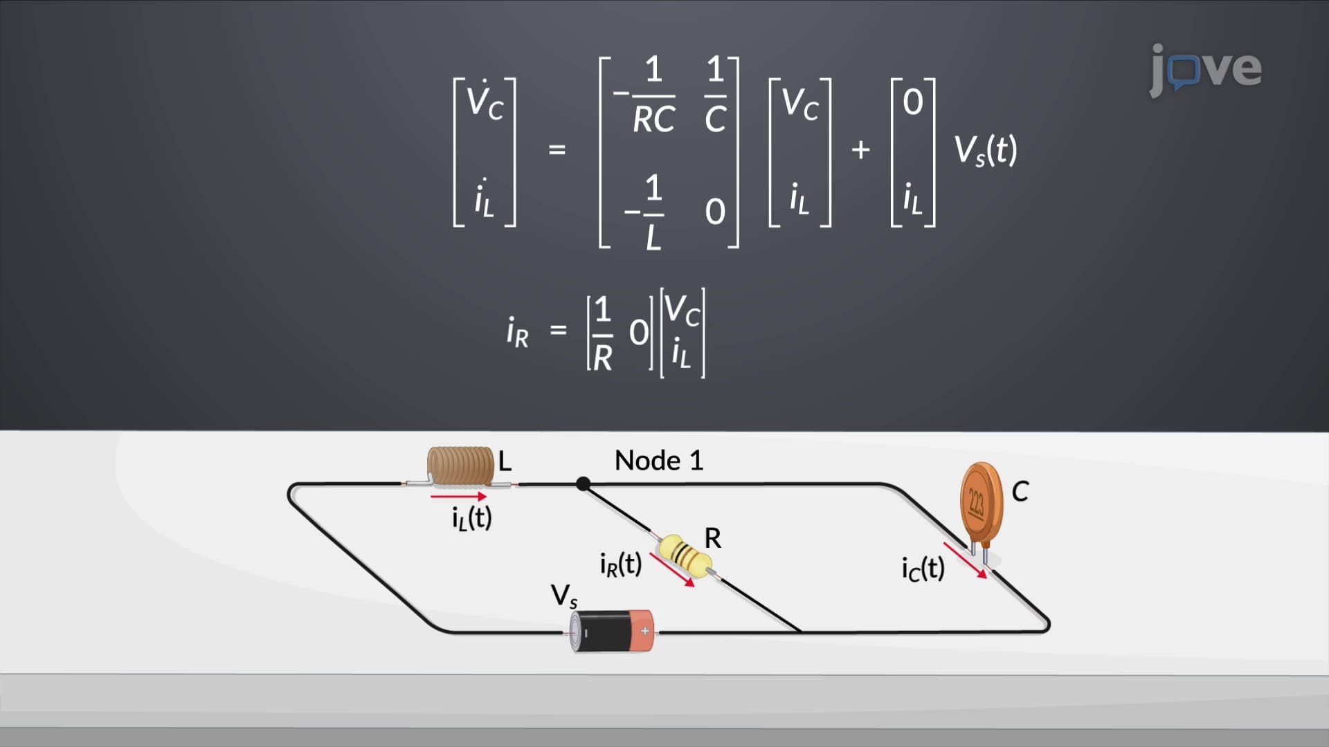

Video Summary: What Is State Space Representation
Ever wonder how NASA engineers control complex spacecraft with multiple thrusters and sensors simultaneously? Converting a transfer function to state space representation unlocks this capability, allowing engineers to handle multi-input, multi-output systems that traditional frequency-domain methods cannot manage. Unlike single-input systems analyzed in typical AP Physics courses, state space representation can model everything from Boeing 787 flight control systems to Tesla's battery management networks. What is state space representation becomes clear when you realize it transforms higher-order differential equations into manageable first-order matrix systems. Watch the full video on JoVE Coach to master this concept with expert-led visuals and step-by-step explanations.
State space representation fundamentally transforms how engineers analyze dynamic systems by converting complex higher-order differential equations into manageable first-order matrix equations. While frequency-domain techniques taught in AP Physics and introductory engineering courses work well for simple, linear systems, state space representation handles the real-world complexity of nonlinear, time-varying, and multiple-input multiple-output (MIMO) systems that dominate modern technology.
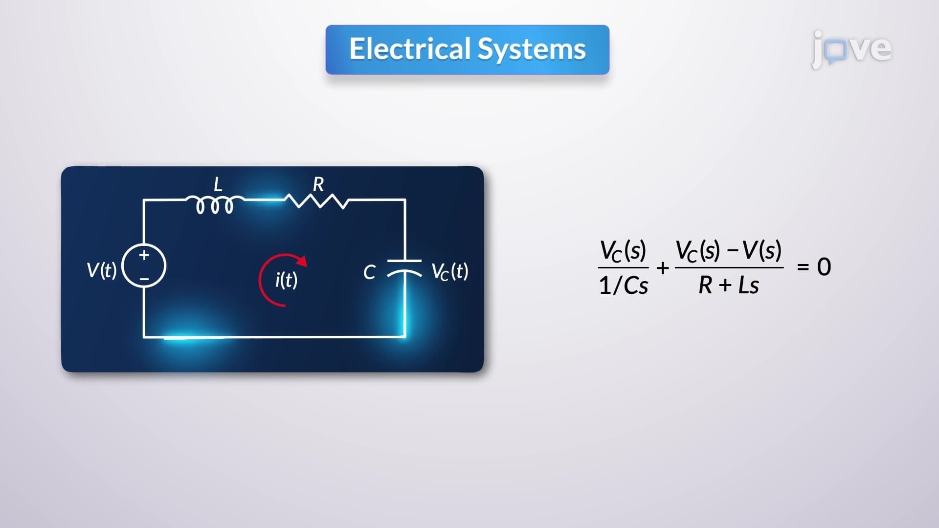
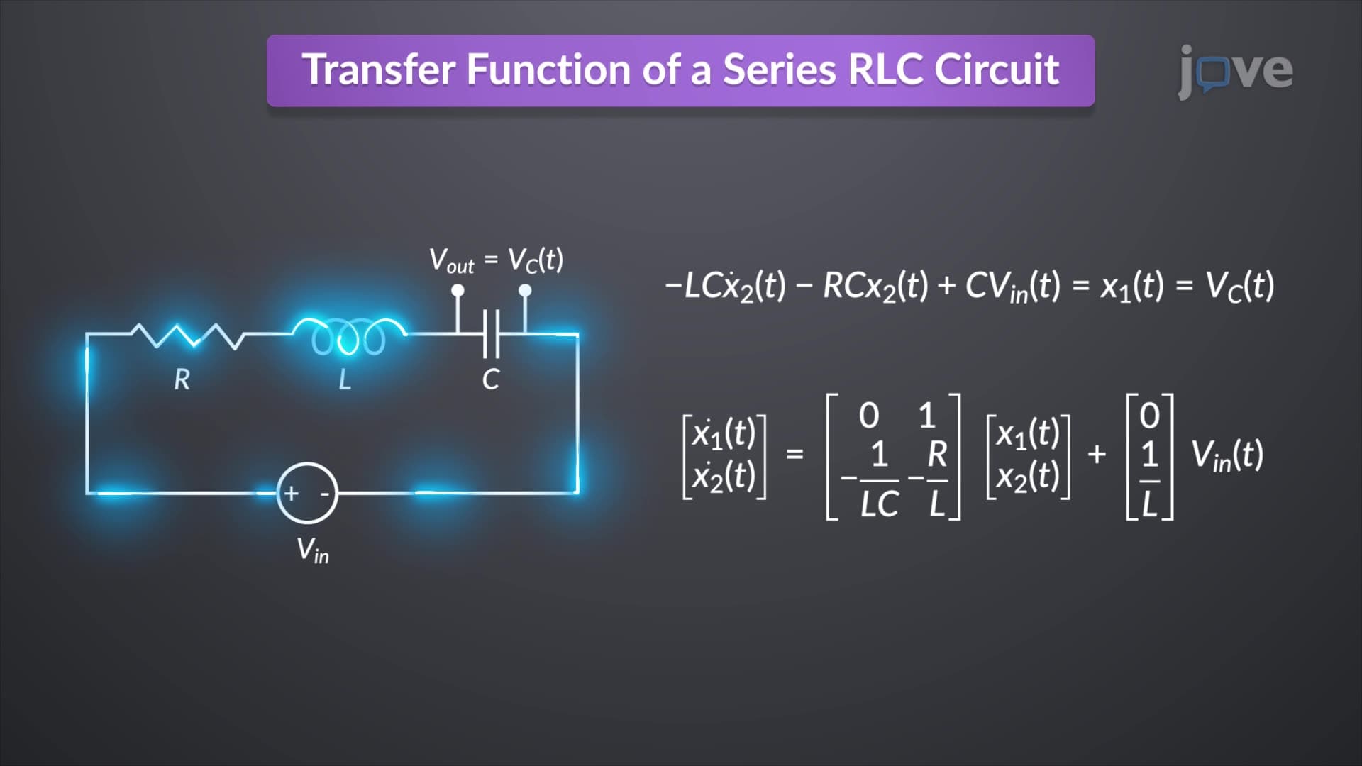
The transition from transfer function to state space begins by identifying state variables-quantities that capture a system's energy storage. In electrical circuits, these are typically capacitor voltages and inductor currents, since capacitors store electric energy and inductors store magnetic energy. For a second-order RLC circuit common in college electronics labs, you need exactly two state variables to completely describe the system's behavior.
This concept appears frequently on the Fundamentals of Engineering (FE) exam and advanced placement tests. Students learning transfer function to state space conversion discover that state variables must be linearly independent and sufficient to determine the system's future behavior given current inputs.
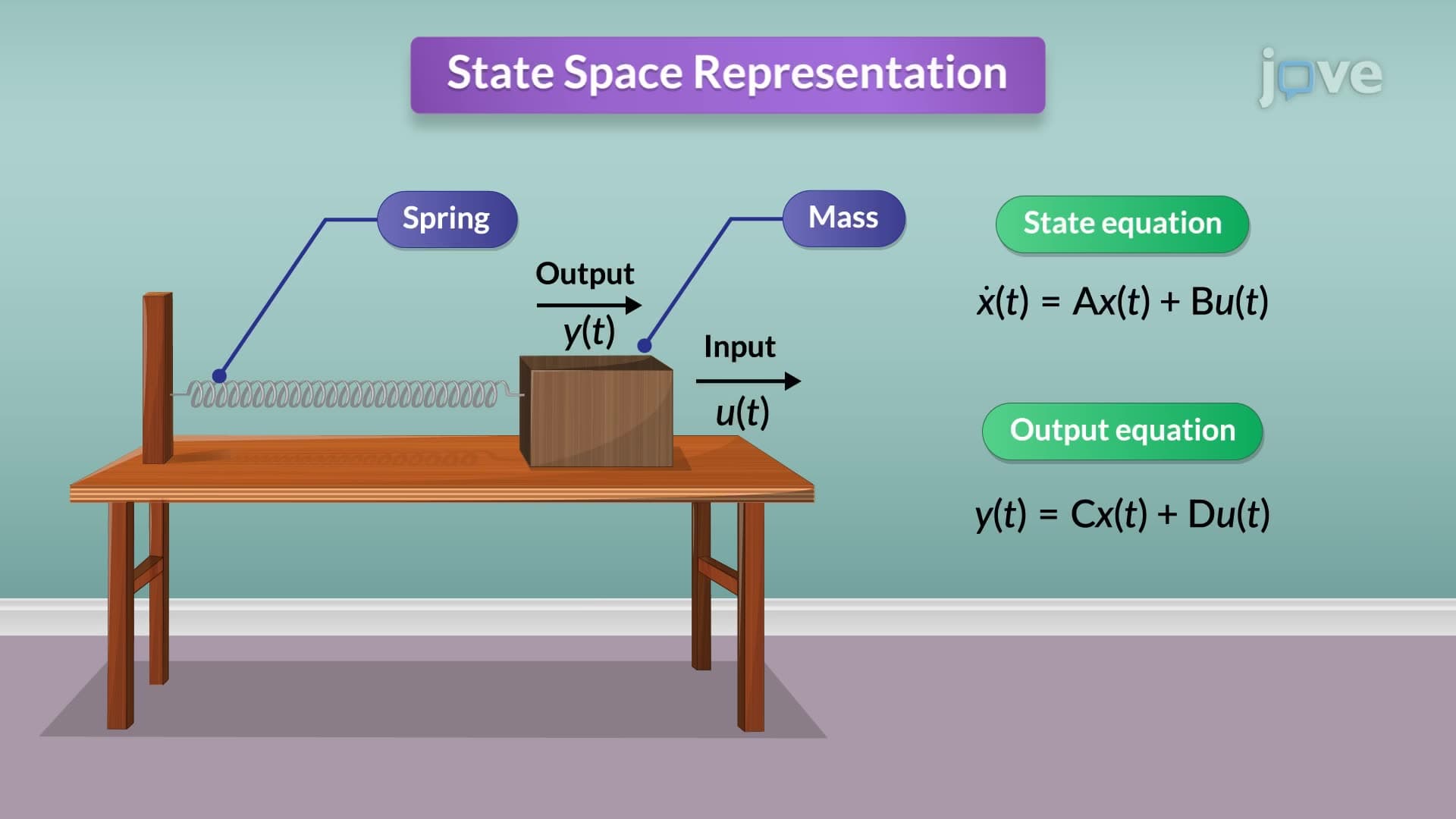
State space representation expresses system dynamics as x'(t) = Ax(t) + Bu(t) and outputs as y(t) = Cx(t) + Du(t), where x represents state variables, u inputs, and y outputs. This matrix form enables computer analysis of complex systems like automotive engine control units, which simultaneously manage fuel injection, ignition timing, and emissions control.
Boeing's 737 MAX flight control system exemplifies practical state space applications, where multiple sensors and actuators work together. Unlike simple transfer function analysis taught in introductory control systems courses, state space methods can handle these interconnected, multi-variable systems that characterize modern aerospace and automotive technologies.
Understanding transfer function to state space conversion prepares students for advanced coursework in mechanical, electrical, and aerospace engineering programs. MIT's undergraduate control systems curriculum emphasizes state space methods because they provide the foundation for modern control theory, optimal control, and state estimation techniques essential in robotics, autonomous vehicles, and smart grid systems.
Related Micro-courses