Loading video…


 12 Concepts
 9.6K views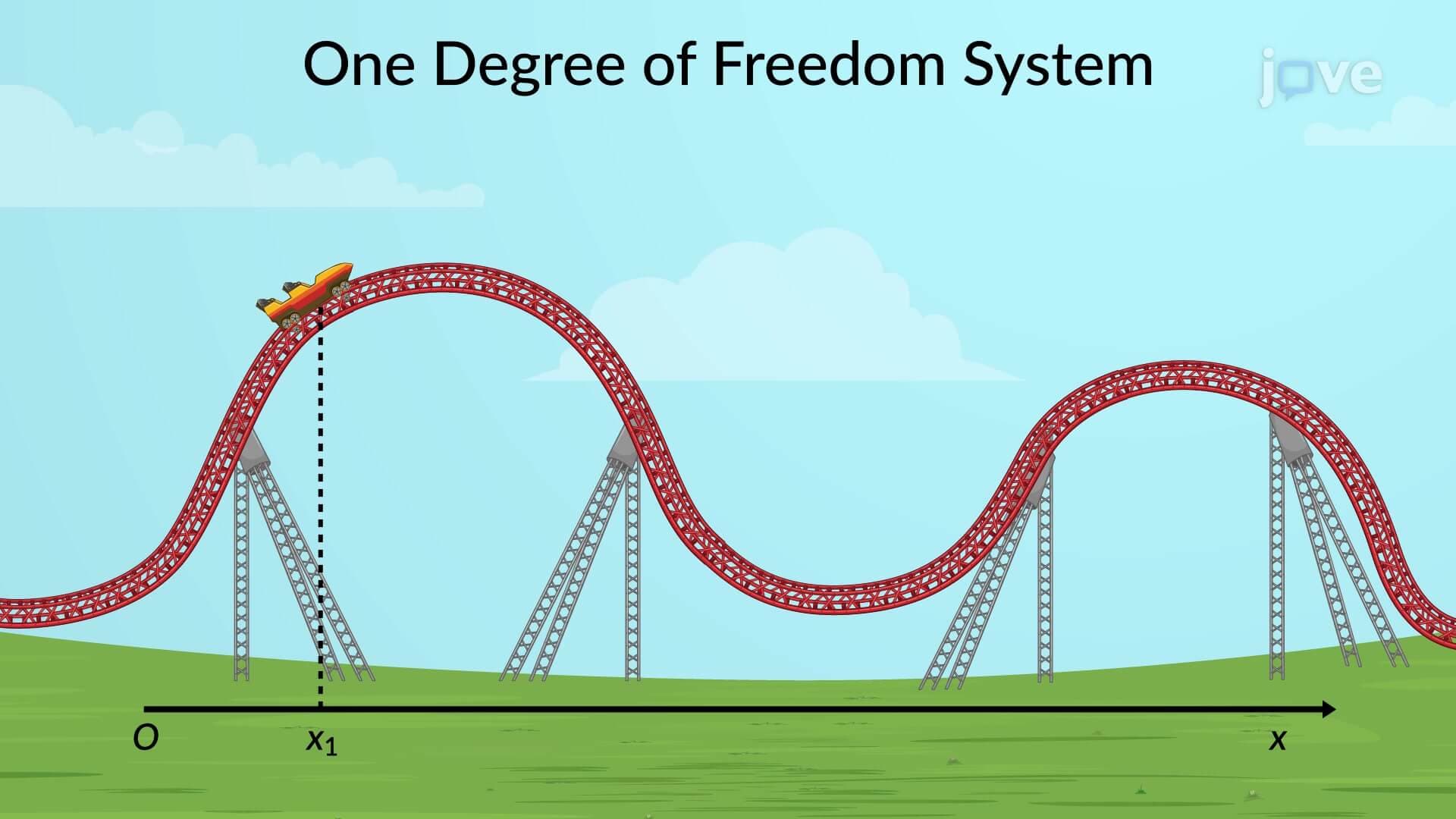

Video Summary: One Degree of Freedom System Explained
Ever wonder why a pendulum clock keeps perfect time or how engineers predict when a building will sway dangerously in wind? A one degree of freedom system requires just one variable to describe its complete motion, making it the foundation for understanding complex mechanical behaviors. From the Golden Gate Bridge's calculated oscillations to a simple swing set in any US playground, these systems follow predictable patterns based on their potential energy landscapes. Watch the full video on JoVE Coach to master this concept with expert-led visuals and step-by-step explanations.
A one degree of freedom system represents the simplest form of mechanical analysis, where a single coordinate completely describes the system's configuration. This foundational concept appears throughout physics and engineering curricula, from AP Physics courses to university-level mechanical engineering programs. Unlike complex systems requiring multiple variables, these systems offer clear insights into fundamental mechanical principles that students encounter on standardized tests like the MCAT and AP Physics exams.
The relationship between potential energy and system position forms the cornerstone of stability analysis. When plotting potential energy against the single degree of freedom variable, equilibrium occurs where the slope equals zero-mathematically expressed as dU/dx = 0, where U represents potential energy and x represents the position variable. This principle directly applies to problems students encounter in college physics courses and professional engineering licensing exams.
Consider the Golden Gate Bridge's main cables: each cable segment can be analyzed as a one degree of freedom system where the vertical displacement represents the single variable. Engineers use potential energy functions to predict how these cables respond to varying loads, ensuring structural integrity under different conditions.
The second derivative test provides a powerful tool for classifying equilibrium stability. When d²U/dx² > 0, the system exhibits stable equilibrium-like a ball resting at the bottom of a bowl. The positive second derivative indicates a potential energy minimum, meaning small disturbances cause restoring forces that return the system to equilibrium.
Conversely, when d²U/dx² < 0, unstable equilibrium occurs-imagine balancing a pencil on its point. The negative second derivative represents a potential energy maximum, where slight disturbances cause the system to move away from equilibrium. This concept frequently appears in MCAT physics sections and engineering dynamics courses.
When the second derivative equals zero, higher-order derivatives determine stability. If the first non-zero derivative has even order and positive value, stable equilibrium exists. However, if this derivative has negative value (regardless of order) or positive odd order, instability results. Neutral equilibrium occurs when all higher-order derivatives equal zero, creating a flat potential energy landscape-like a ball on a perfectly flat table.
These mathematical principles directly translate to practical applications in aerospace engineering, where spacecraft attitude control systems rely on understanding equilibrium stability for mission success.
Related Micro-courses