Loading video…


 14 Concepts
 114.6K views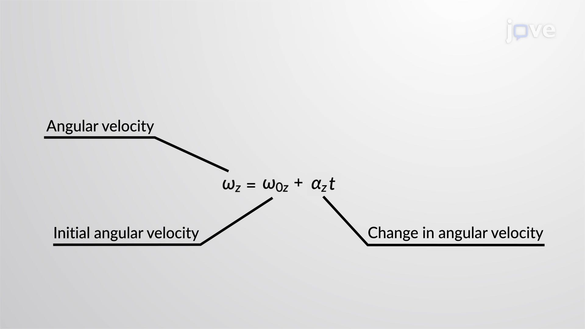

Video Summary: Rotation with Constant Angular Acceleration I Explained
Did you know that a figure skater's spinning speed follows the same mathematical principles as a car accelerating down a highway? Rotation with constant angular acceleration I reveals how rotational motion mirrors linear motion through parallel kinematic equations. Just like NASA engineers calculate spacecraft rotational maneuvers using these exact principles, students can master rotational dynamics by understanding how angular velocity, acceleration, and displacement connect mathematically. Rotation With Constant Angular Acceleration I Explained transforms complex rotational concepts into manageable equations that apply from spinning turbines to planetary motion. Watch the full video on JoVE Coach to master this concept with expert-led visuals and step-by-step explanations.
Rotation with constant angular acceleration represents one of physics' most elegant parallels between linear and rotational motion. When an object rotates with unchanging angular acceleration, its motion follows predictable mathematical relationships that mirror familiar linear kinematic equations. This concept forms the foundation for analyzing everything from electric motor startup sequences to satellite orientation maneuvers.
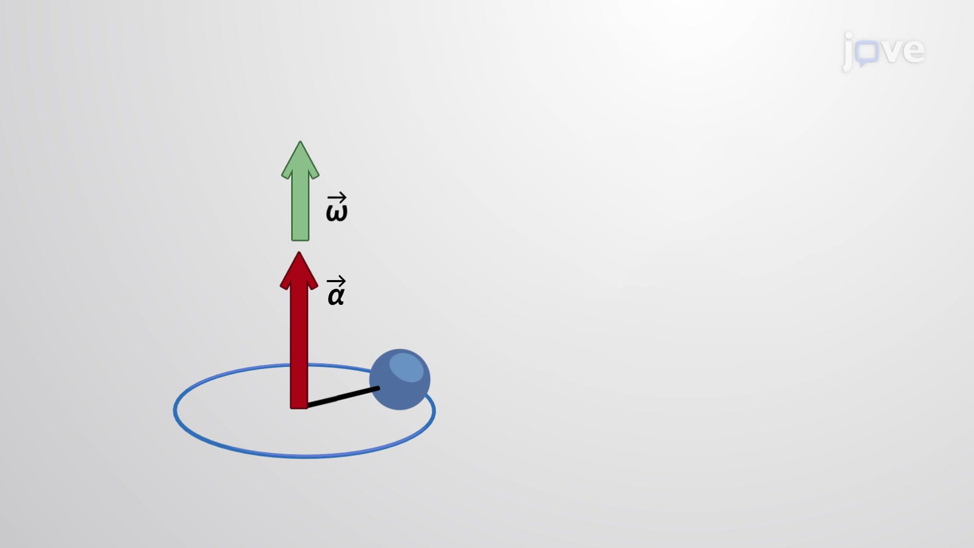
The beauty of rotational kinematics lies in its direct correspondence to linear motion. Where linear motion uses position (x), velocity (v), and acceleration (a), rotational motion employs angular position (θ), angular velocity (ω), and angular acceleration (α). This parallel structure means students already familiar with linear kinematics can rapidly master rotational concepts by recognizing these analogies.
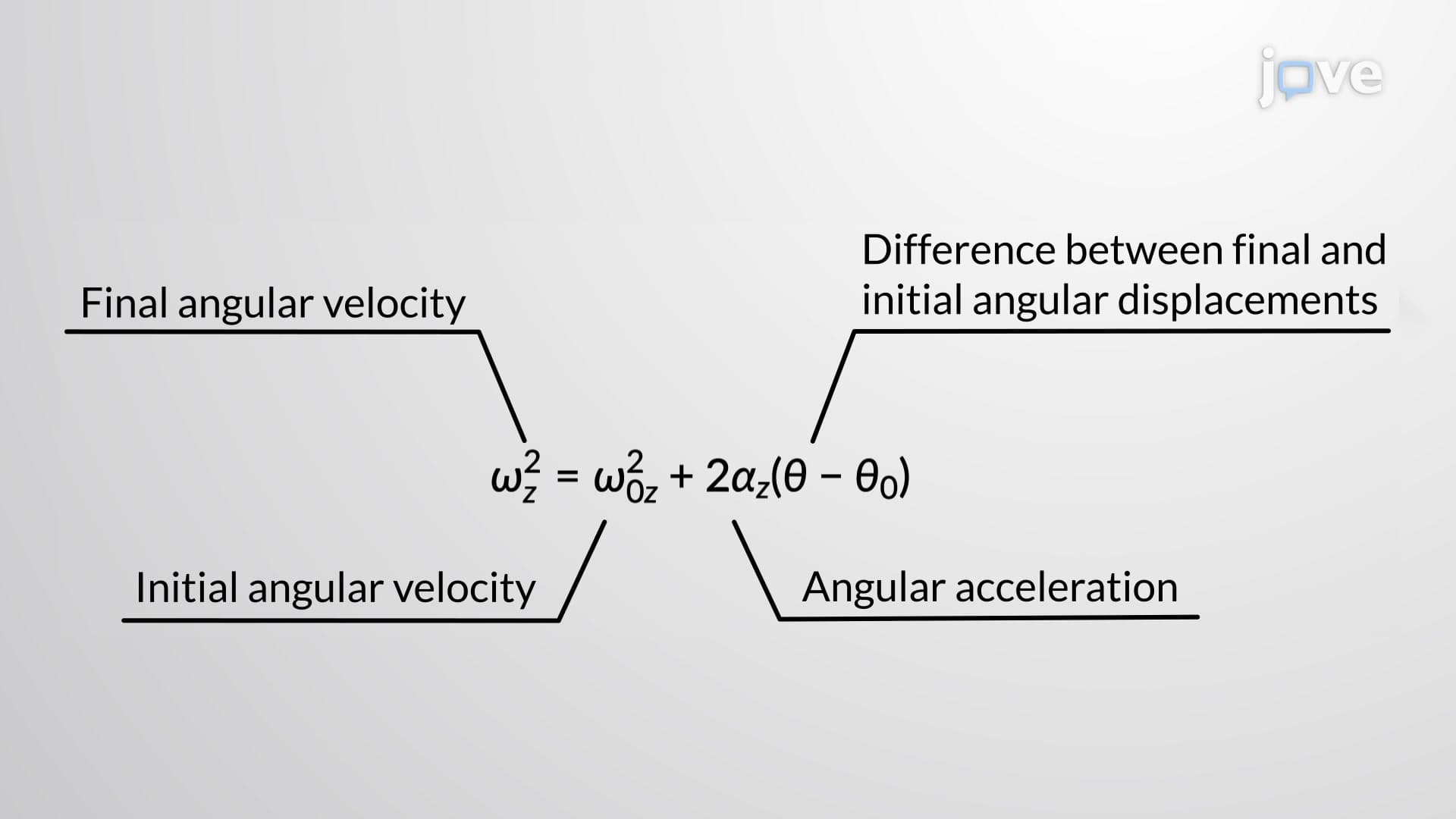
Three fundamental equations govern rotation with constant angular acceleration. The first equation, ω = ω₀ + αt, calculates final angular velocity by adding initial angular velocity to the change in velocity over time. This equation proves invaluable when analyzing how quickly turbines reach operating speeds or how long spacecraft take to achieve desired rotation rates.
The second equation, θ = θ₀ + ω₀t + (1/2)αt², determines angular displacement over time. Engineers use this relationship when programming robotic arms or calculating satellite positioning requirements. The equation accounts for both constant rotation and acceleration-induced displacement changes.
American manufacturing relies heavily on rotational motion principles. Consider a wind turbine generator starting from rest: engineers must calculate how long the turbine takes to reach optimal rotation speed given wind conditions and mechanical constraints. Similarly, automotive engineers analyze engine crankshaft acceleration during startup to optimize fuel injection timing and reduce emissions.
For AP Physics and college-level courses, problems typically involve multiple-step calculations combining different kinematic equations. Students might calculate how many revolutions a spinning wheel makes while slowing to a stop, or determine the angular acceleration needed for a satellite to complete a specific rotational maneuver within a given timeframe. Success requires identifying known variables, selecting appropriate equations, and maintaining consistent units throughout calculations.
MCAT and engineering exam questions frequently test rotational kinematics through biomedical applications like centrifuge operation or MRI scanner rotation. These problems require understanding when constant angular acceleration assumptions remain valid and recognizing limitations in real-world systems where friction and other forces may cause varying acceleration rates.
Related Micro-courses