Loading subject page…


72,639 views


Video Summary: What Is Precipitation Titration Curve Analysis
Ever wonder how forensic labs determine chloride levels in blood samples or how the EPA monitors silver contamination in water supplies? Precipitation titration curve analysis reveals the dramatic concentration changes that occur when ions form insoluble compounds during titration. This analytical technique helps chemists identify equivalence points by tracking how metal ion concentrations shift as precipitates form and dissolve. Understanding what precipitation titration curve analysis involves is crucial for quantitative chemistry success. Watch the full video on JoVE Coach to master this concept with expert-led visuals and step-by-step explanations.
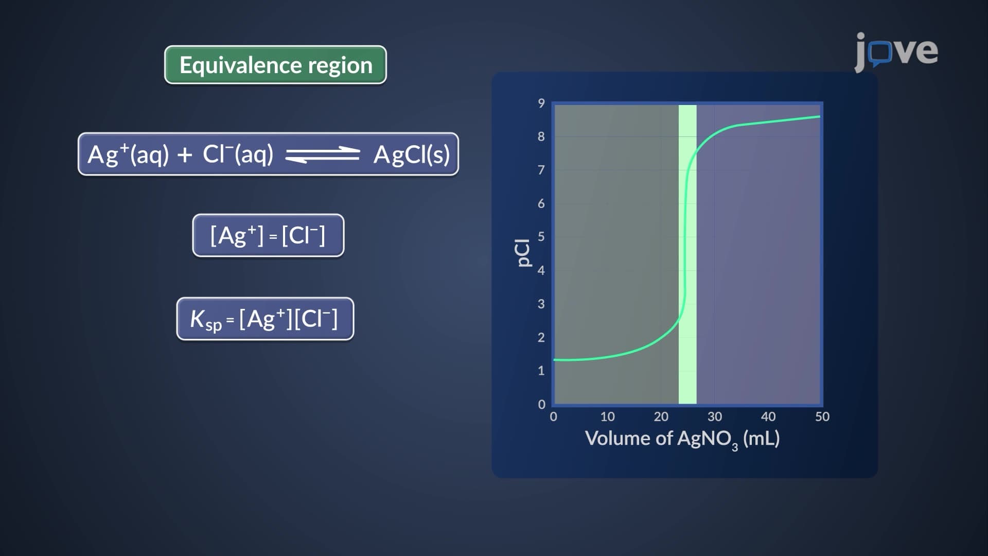
Precipitation titration curve analysis involves plotting the concentration of a metal ion (typically expressed as pAg for silver) against the volume of titrant added during a precipitation reaction. Unlike pH curves in acid-base titrations, these curves track the formation and dissolution of sparingly soluble ionic compounds. The dramatic concentration changes near equivalence points make these curves powerful tools for quantitative analysis.
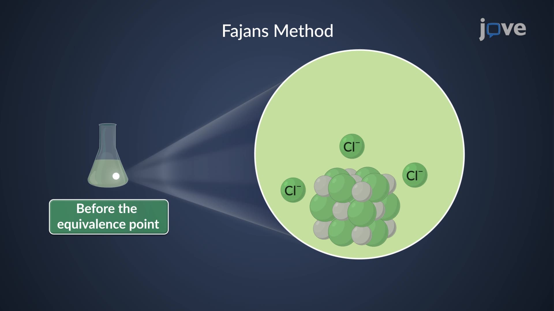
The shape of these curves depends heavily on the solubility product constant (Ksp) of the precipitate formed. When silver nitrate titrates chloride ions, the initial silver concentration remains extremely low because any silver added immediately precipitates as AgCl. This creates a relatively flat region at the curve's beginning, where pAg values remain high (low [Ag+]).
At the equivalence point, all chloride has been consumed, and the next drop of silver nitrate causes a sharp rise in silver ion concentration. This creates the characteristic steep inflection that defines the equivalence point in precipitation curve analysis. The magnitude of this jump correlates directly with the Ksp value-compounds with lower solubility products produce more dramatic concentration changes.
Silver iodide (Ksp = 8.5 × 10⁻¹⁷) creates sharper breaks than silver chloride (Ksp = 1.8 × 10⁻¹⁰) because its lower solubility means even smaller amounts of excess silver produce detectable concentration increases. This principle helps analytical chemists choose appropriate titration conditions for maximum precision.
When analyzing mixtures containing both iodide and chloride, precipitation titration curve analysis reveals two distinct equivalence points. Silver iodide forms first due to its lower Ksp, consuming all available iodide before chloride precipitation begins. The resulting curve shows two separate inflection points, allowing simultaneous determination of both halides in a single analysis.
This sequential precipitation principle applies broadly in environmental analysis. The EPA uses similar techniques to monitor heavy metal contamination in water supplies, where different metals precipitate at characteristic pH or reagent concentrations. Understanding these curves helps environmental scientists identify and quantify multiple contaminants simultaneously.
Major US clinical laboratories routinely use precipitation curve analysis for chloride determinations in blood and urine samples. The Cleveland Clinic and Mayo Clinic laboratories rely on automated argentometric analyzers that generate real-time precipitation curves for quality control. These instruments can detect chloride levels as low as 10 mg/L, crucial for diagnosing electrolyte imbalances.
Students preparing for AP Chemistry exams frequently encounter precipitation curve problems, particularly in the equilibrium and analytical chemistry sections. The MCAT also tests this concept in its Chemical and Physical Foundations section, often combining precipitation curves with Le Chatelier's principle and solubility equilibria concepts.
Related Micro-courses