Loading video…


 14 Concepts
 173.2K views

Video Summary: What Is Normal Distribution
Did you know that SAT scores, heights of American teenagers, and even the diameter of M&M candies all follow the same mathematical pattern? Normal distribution forms the backbone of statistics, appearing everywhere from college entrance exam scores to medical research. This bell-shaped probability distribution, defined by its mean and standard deviation, helps us understand how data clusters around average values. For instance, if the average birth weight of babies in US hospitals is 7.7 pounds with predictable variation, we can calculate the probability of any specific weight range. Watch the full video on JoVE Coach to master this concept with expert-led visuals and step-by-step explanations.
Normal distribution represents one of the most important concepts in statistics, forming the foundation for countless applications in science, business, and standardized testing. This continuous probability distribution creates a symmetric, bell-shaped curve that describes how data points cluster around a central value. Unlike discrete distributions that deal with specific outcomes, normal distribution deals with ranges of continuous values, making it perfect for measuring phenomena like height, weight, test scores, and measurement errors.
The mathematical beauty of normal distribution lies in its universality. Whether you're analyzing ACT scores across American high schools, measuring the effectiveness of a new medication in clinical trials, or studying manufacturing tolerances at Ford Motor Company, the same underlying pattern emerges. This consistency allows statisticians and researchers to make powerful predictions about populations based on sample data.
Named after German mathematician Carl Friedrich Gauss, the normal distribution follows a specific mathematical formula that depends on just two parameters: the mean (μ) and standard deviation (σ). The mean determines where the center of the bell curve sits on the horizontal axis, while the standard deviation controls how spread out the data points are from that center.
In practical terms, consider SAT Math scores, which follow a normal distribution with a mean of approximately 528 and standard deviation of 120. This means most students score near 528, with fewer students achieving very high or very low scores. The standard deviation tells us that about 68% of students score between 408 and 648 (within one standard deviation), while 95% score between 288 and 768 (within two standard deviations).
The concept of standard normal distribution revolutionizes how we work with normally distributed data. By converting any normal distribution to have a mean of 0 and standard deviation of 1, we create a universal reference system. This transformation uses z-scores, calculated as z = (x - μ)/σ, where x is any data point, μ is the mean, and σ is the standard deviation.
This standardization proves invaluable for AP Statistics students and college-level coursework. Instead of memorizing probability tables for countless different normal distributions, students only need to reference one standard normal table. For example, whether you're analyzing birth weights, reaction times in psychology experiments, or quality control measurements in pharmaceutical manufacturing, the z-score transformation allows you to use the same probability calculations.
Normal distribution appears extensively in standardized tests like the MCAT, where understanding statistical concepts is crucial for interpreting research data. Medical school applicants encounter normal distribution in contexts ranging from analyzing drug effectiveness to interpreting diagnostic test results. The concept also features prominently in AP Statistics curriculum, where students learn to identify normal patterns in real datasets and calculate probabilities for specific ranges.
In professional settings, normal distribution assumptions underlie many statistical tests used in clinical research, market analysis, and quality control. Understanding when data follows a normal distribution-and when it doesn't-becomes critical for making valid statistical inferences and avoiding common analytical mistakes.
Related Micro-courses