Loading concepts…


15 Concepts
15 Concepts
13 Concepts
11 Concepts
9 Concepts
14 Concepts
11 Concepts
15 Concepts
13 Concepts
7 Concepts
10 Concepts
10 Concepts
22 Concepts
19 Concepts
16 Concepts
16 Concepts
7 Concepts
 13 Concepts
 130.6K Views
 Popular topics






Hypothesis testing is a fundamental statistical method used to make evidence-based decisions about population characteristics. Through JoVE Coach's comprehensive micro-course, students learn to formulate null and alternative hypotheses, calculate test statistics, interpret p-values, and apply various testing methods including z-tests and t-tests across diverse scientific and business applications.
1. Hypothesis Formulation and Types Understanding how to construct testable statements about population characteristics forms the foundation of statistical inference. A hypothesis differs from predictions or assumptions by making general claims about patterns rather than specific cause-and-effect relationships. Students learn to distinguish between research hypotheses (what researchers believe) and statistical hypotheses (null and alternative statements). For example, when testing whether a new SAT prep course improves scores, the null hypothesis states no difference exists, while the alternative suggests improvement occurs. This concept applies across disciplines, from medical research testing drug effectiveness to business studies examining consumer preferences.
2. Null and Alternative Hypotheses Every hypothesis test requires two competing statements: the null hypothesis (H₀) representing no effect or no difference, and the alternative hypothesis (H₁) representing the research claim. The null hypothesis always contains equality (=, ≤, ≥), while alternatives use inequality symbols (<, >, ≠). In quality control testing at a pharmaceutical company, H₀ might state that medication potency equals 100mg, while H₁ suggests it differs from 100mg. The alternative hypothesis determines test direction: right-tailed tests examine increases, left-tailed tests check decreases, and two-tailed tests detect any difference. This framework ensures objective testing by assuming no effect until evidence proves otherwise.
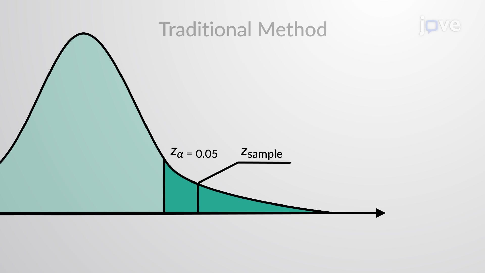
3. Test Statistics and Critical Regions Converting sample data into standardized test statistics enables comparison across different studies and parameters. The test statistic (z, t, or χ²) measures how many standard errors the sample result falls from the hypothesized population value. Critical regions represent areas under probability curves where test statistics lead to null hypothesis rejection. For instance, when testing whether average student loan debt exceeds $30,000 using a significance level of 0.05, the critical region occupies the right tail containing the most extreme 5% of possible z-values. Critical values serve as boundaries separating rejection and non-rejection regions, providing clear decision rules for researchers.
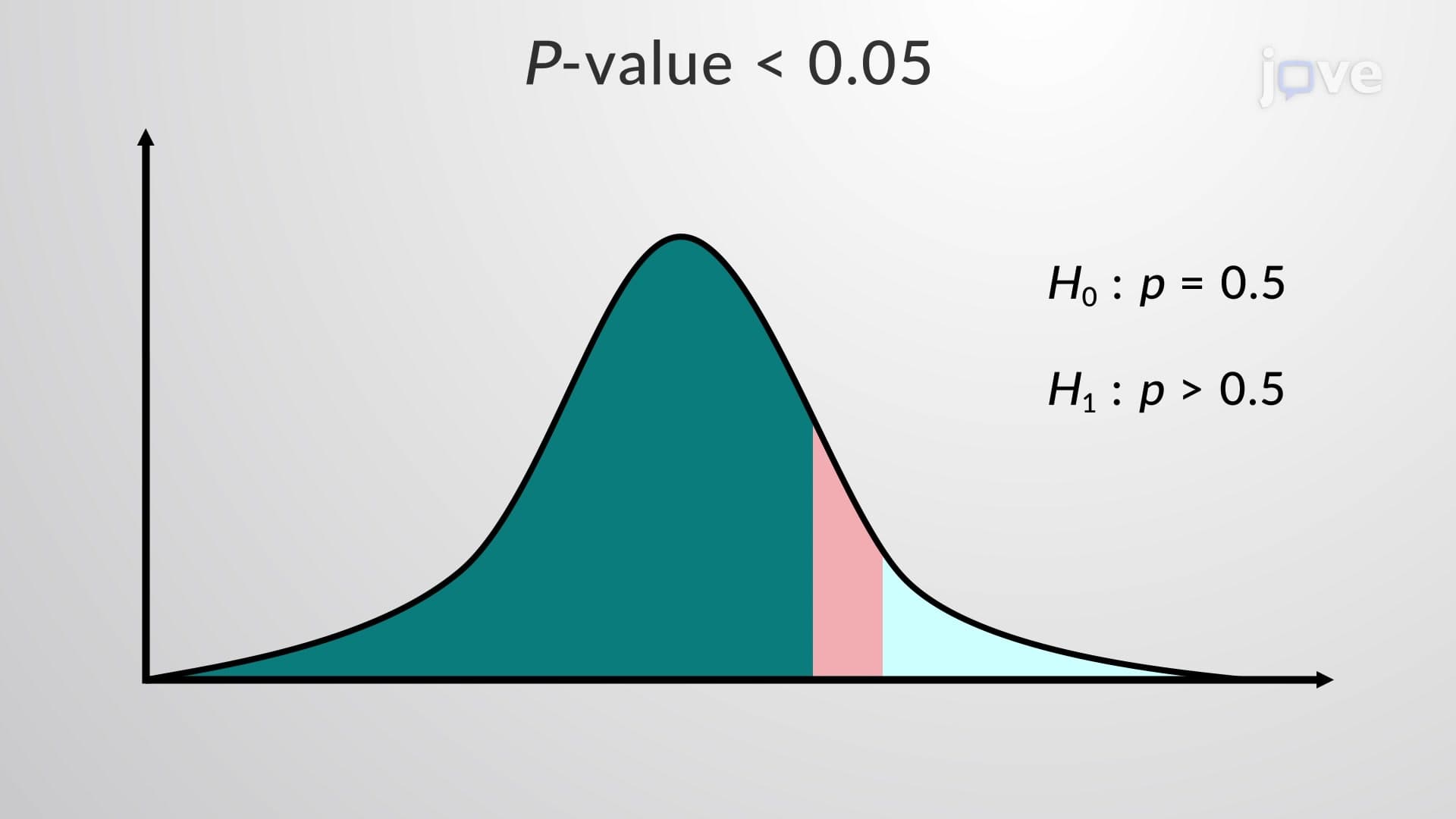
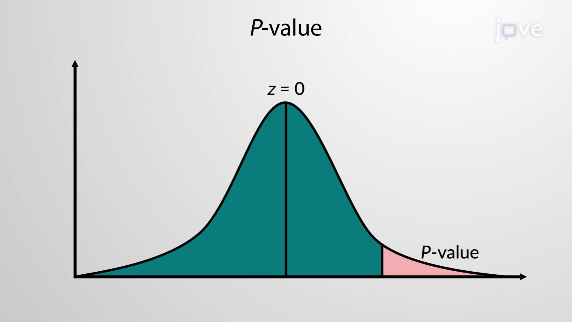
4. P-values and Statistical Significance The p-value quantifies evidence against the null hypothesis by calculating the probability of observing results at least as extreme as those obtained, assuming H₀ is true. Smaller p-values indicate stronger evidence against the null hypothesis. When comparing p-values to predetermined significance levels (commonly α = 0.05), researchers make objective decisions: p ≤ α leads to rejection, while p > α results in failure to reject H₀. In clinical trials testing new treatments, a p-value of 0.02 suggests only 2% probability that observed improvements occurred by chance alone. This method provides more nuanced interpretation than simple reject/don't reject decisions, allowing researchers to assess evidence strength on a continuous scale.
5. Types of Hypothesis Tests The direction of the research question determines whether to conduct one-tailed or two-tailed tests. Right-tailed tests examine claims about increases (H₁: parameter > value), such as testing whether a training program improves employee productivity above current levels. Left-tailed tests investigate decreases (H₁: parameter < value), like determining if a new manufacturing process reduces defect rates below existing standards. Two-tailed tests detect any difference (H₁: parameter ≠ value), appropriate when researchers suspect change but don't predict direction, such as studying whether class size affects test scores without knowing if larger or smaller classes perform better. Test choice affects critical regions and p-value calculations.
6. Decision-Making Methods Two primary approaches exist for hypothesis testing decisions: the traditional critical value method and the modern p-value method. The traditional approach compares calculated test statistics to critical values, rejecting H₀ when statistics fall in critical regions. The p-value method compares calculated p-values to significance levels, offering more flexibility and detailed information about evidence strength. In educational research testing whether online learning improves standardized test scores, both methods reach identical conclusions but provide different insights. The p-value method has gained popularity because it reports exact probability levels rather than simple reject/don't reject decisions, enabling readers to judge evidence strength independently.
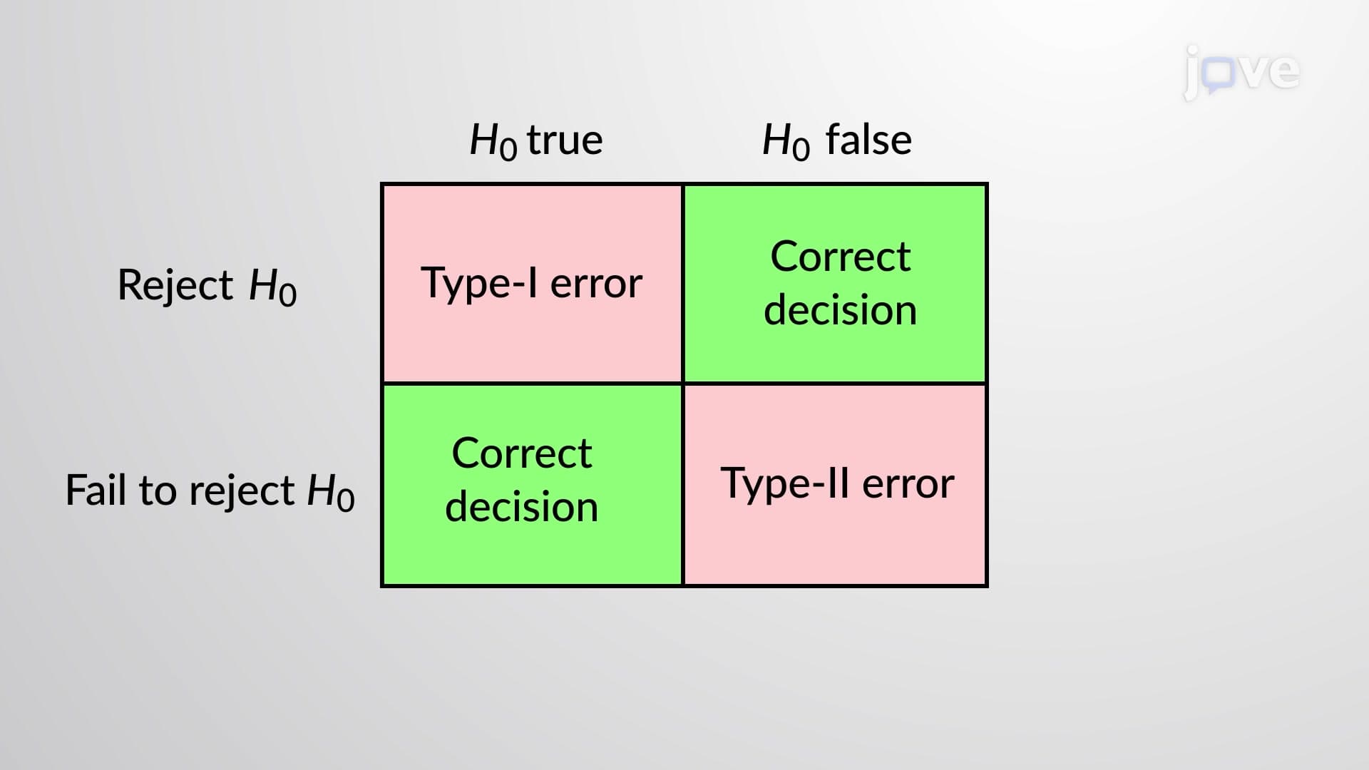
7. Statistical Errors in Hypothesis Testing Hypothesis testing involves two potential errors with different consequences. Type I error occurs when researchers reject true null hypotheses, similar to false positive medical test results. The probability of Type I error equals the significance level (α), typically set at 0.05. Type II error happens when researchers fail to reject false null hypotheses, resembling false negative test results. Type II error probability (β) depends on effect size, sample size, and significance level. In pharmaceutical testing, Type I errors might approve ineffective drugs, while Type II errors could reject beneficial treatments. Understanding these errors helps researchers choose appropriate significance levels and sample sizes, balancing risks of incorrect decisions in their specific contexts.
8. Testing Population Proportions When research questions involve categorical data and population proportions, specific testing procedures apply. These tests use the normal approximation to binomial distribution when sample sizes meet certain conditions (np ≥ 5 and n(1-p) ≥ 5). For example, testing whether more than 60% of college students work part-time jobs involves calculating a z-statistic using sample proportion, hypothesized proportion, and standard error. The test statistic follows: z = (p̂ - p₀) / √[p₀(1-p₀)/n]. Applications include market research studying brand preferences, political polling examining candidate support, and quality control testing defect rates. Results help organizations make data-driven decisions about marketing strategies, policy changes, or process improvements.
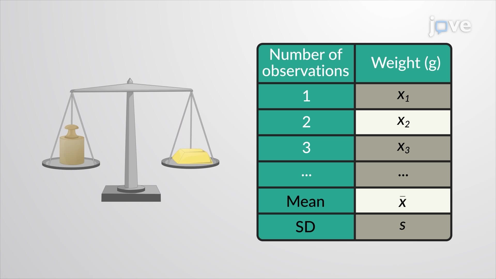
9. Testing Population Means Mean testing procedures vary depending on whether population standard deviation is known or unknown. When σ is known (often from historical data), z-tests apply using the standard normal distribution. Unknown σ situations require t-tests using sample standard deviation and t-distribution. For instance, testing whether a new teaching method increases average math scores involves different approaches: z-test if previous score variability is established, t-test if variability is unknown. The t-distribution accounts for additional uncertainty from estimating σ, producing wider confidence intervals and more conservative results. Sample size affects t-distribution shape, approaching normal distribution as n increases. These tests appear frequently in educational research, medical studies, and business analytics.
10. Testing Population Standard Deviations Testing claims about population variability uses chi-square (χ²) tests, important in quality control and process improvement contexts. Manufacturing companies often need consistent product specifications, making variability testing crucial. For example, testing whether a new production method reduces weight variation in packaged goods involves χ² statistics calculated as: χ² = (n-1)s²/σ₀². The χ² distribution is asymmetric and depends on degrees of freedom (n-1). These tests help determine if process improvements actually reduce variability or if observed changes result from sampling variation. Applications include pharmaceutical manufacturing ensuring consistent drug concentrations, automotive testing examining part tolerances, and service industries monitoring response time consistency.