Measure of Central Tendency

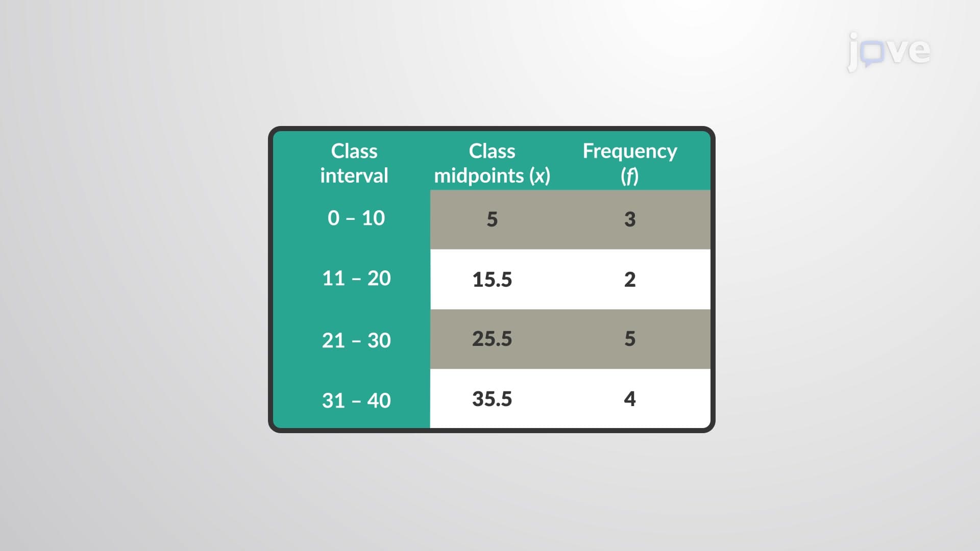
A measure of central tendency identifies a single representative value from a dataset, essential for statistical analysis across STEM fields and standardized testing. This JoVE Coach micro-course covers mean, median, mode, and midrange calculations, exploring arithmetic, geometric, harmonic, weighted, and trimmed means. Students learn to interpret skewed distributions and apply central tendency measures to real-world scenarios like GPA calculations, income analysis, and scientific data interpretation used in US academic and professional contexts.

• Understand the four essential measures of central tendency: mean, median, mode, and midrange
• Calculate arithmetic mean, geometric mean, harmonic mean, and weighted mean for various datasets
• Learn specialized mean calculations including trimmed mean and root mean square
• Identify mode patterns in categorical and numerical data, including bimodal and multimodal distributions
• Analyze frequency distributions and calculate means from grouped data tables
• Apply median calculations for both odd and even-numbered datasets
• Explore skewness types and their impact on central tendency measure relationships
• Interpret central tendency comparisons to understand data distribution characteristics

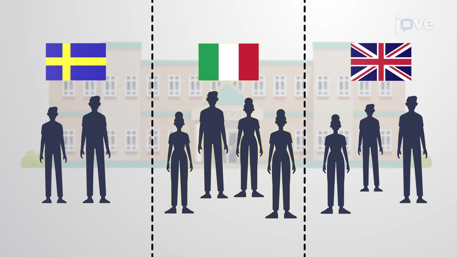
1. Arithmetic Mean and Sample vs Population Distinctions: The most common central tendency measure calculated by summing all values and dividing by the count. Sample mean (x̄) represents data from a subset, while population mean (μ) encompasses entire groups. For example, calculating average SAT scores from 100 students versus all test-takers nationwide. This measure considers every data point but remains sensitive to extreme values, making it less reliable when outliers like unusually high or low test scores skew results significantly.

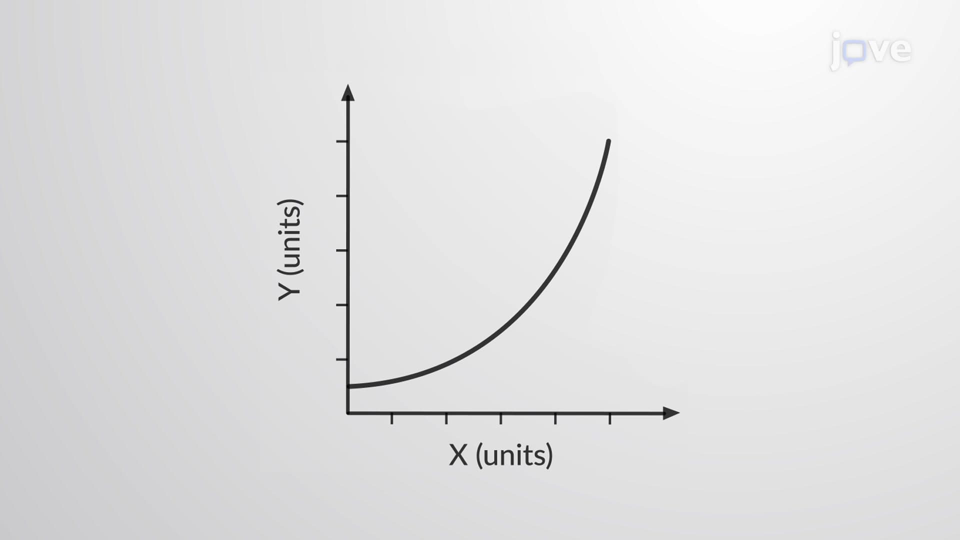
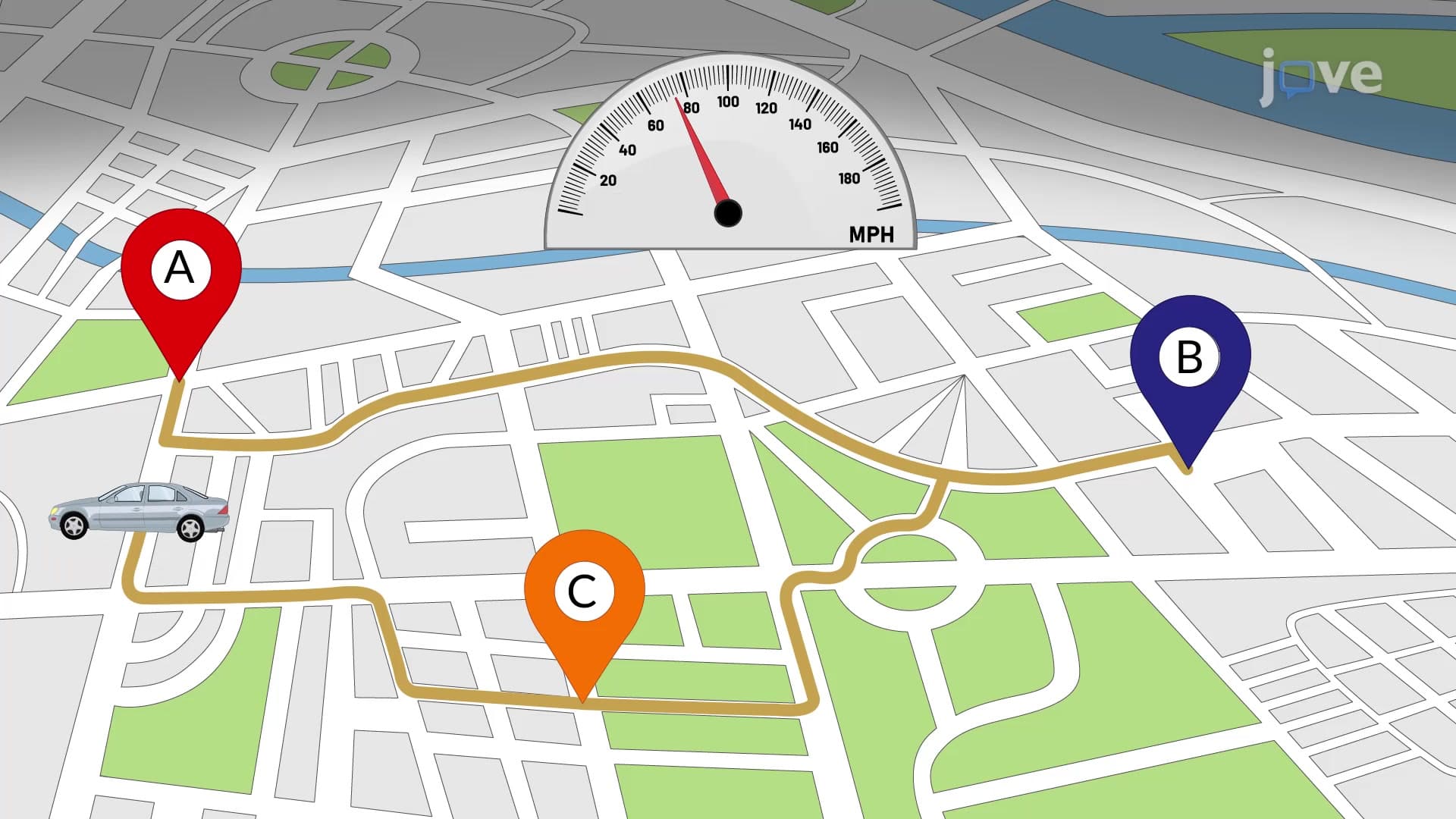
2. Geometric and Harmonic Mean Applications: Geometric mean calculates the nth root of multiplied values, ideal for exponential growth data like population increases or investment returns. Cannot include zero or negative values. Harmonic mean uses reciprocals' arithmetic mean, perfect for rate calculations like average speed during road trips with varying velocities. For instance, driving 30 mph to school, 50 mph home gives a harmonic mean more accurate than simple arithmetic averaging for total trip efficiency.

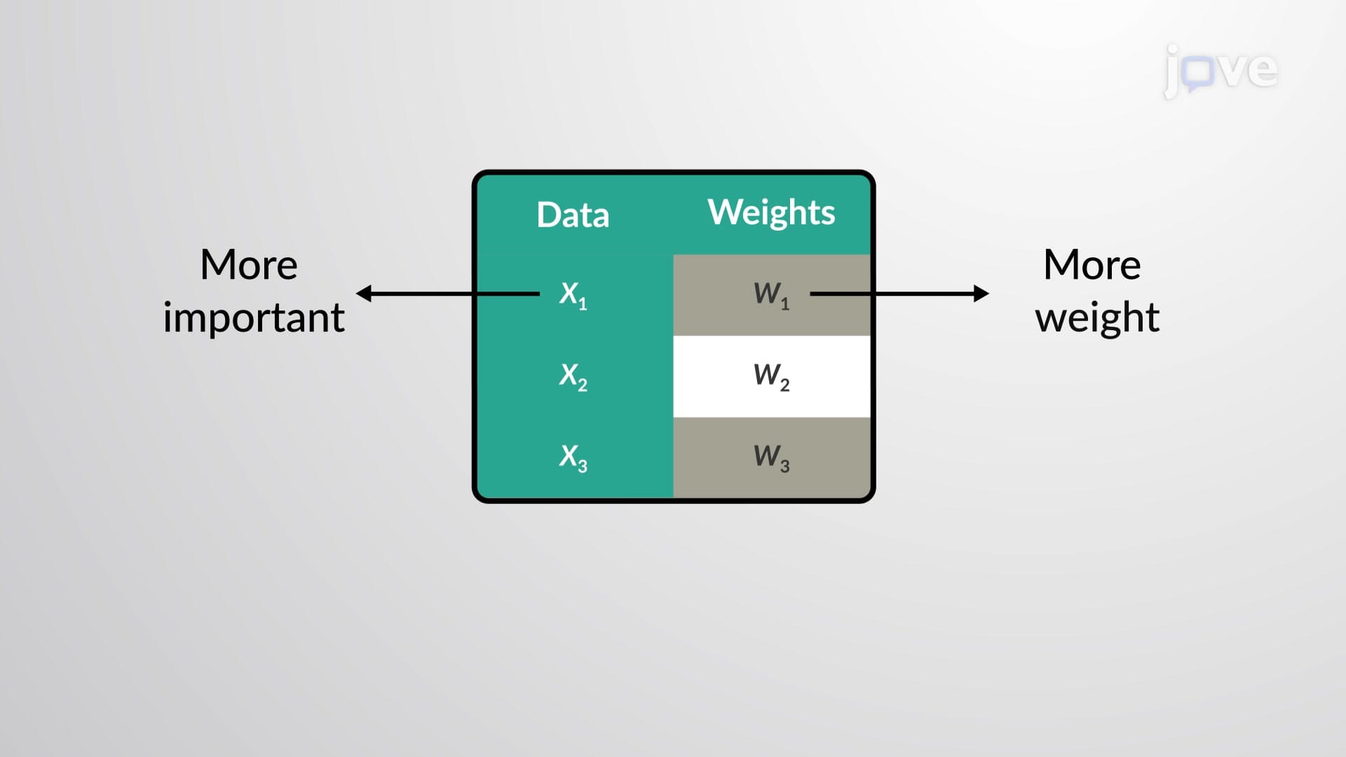
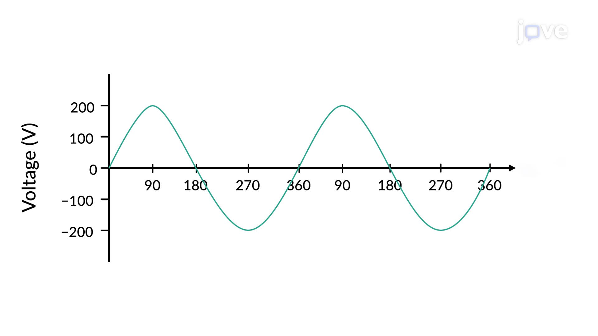
3. Specialized Mean Calculations: Weighted mean multiplies values by importance factors, crucial for GPA calculations where AP courses carry extra weight. Trimmed mean removes extreme values before calculation, like excluding highest/lowest scores to reduce outlier impact. Root mean square handles positive/negative values, essential in physics for AC voltage calculations. These methods provide more accurate central measures when standard arithmetic mean proves inadequate for specific data characteristics.

4. Mode Identification and Distribution Patterns: Mode represents most frequently occurring values, applicable to categorical data like favorite pizza toppings or student majors. Data can be unimodal (one mode), bimodal (two modes), multimodal (multiple modes), or have no mode. Unlike mean and median, mode works with nominal data categories. For example, analyzing most common college entrance exam scores or identifying peak hours for library usage demonstrates mode's practical statistical applications in educational settings.

5. Median Calculation and Resistance to Outliers: Median identifies the middle value in ordered datasets, calculated by arranging data sequentially and finding the center point. With even-numbered datasets, median equals the mean of two middle values. Unlike arithmetic mean, median resists extreme value influence, making it preferable for income analysis where billionaires skew averages. For instance, median household income better represents typical American families than mean income affected by ultra-wealthy outliers.

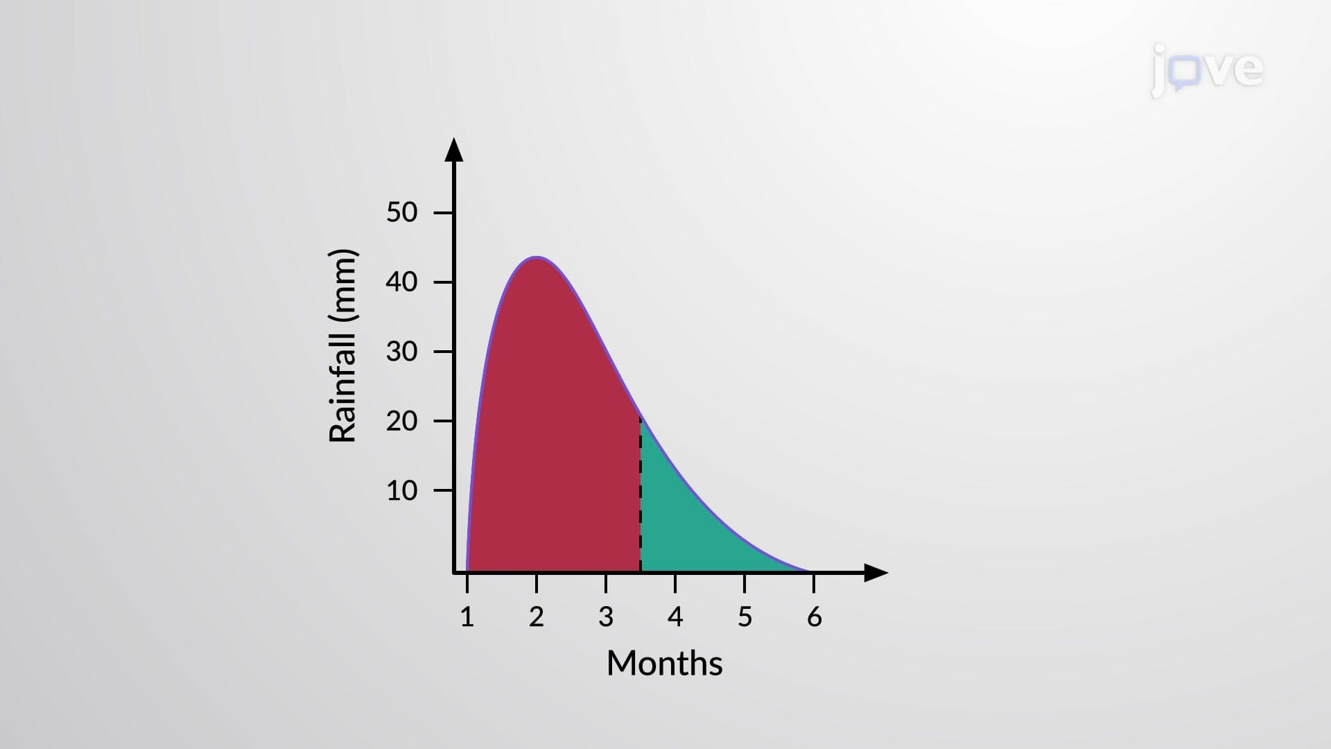
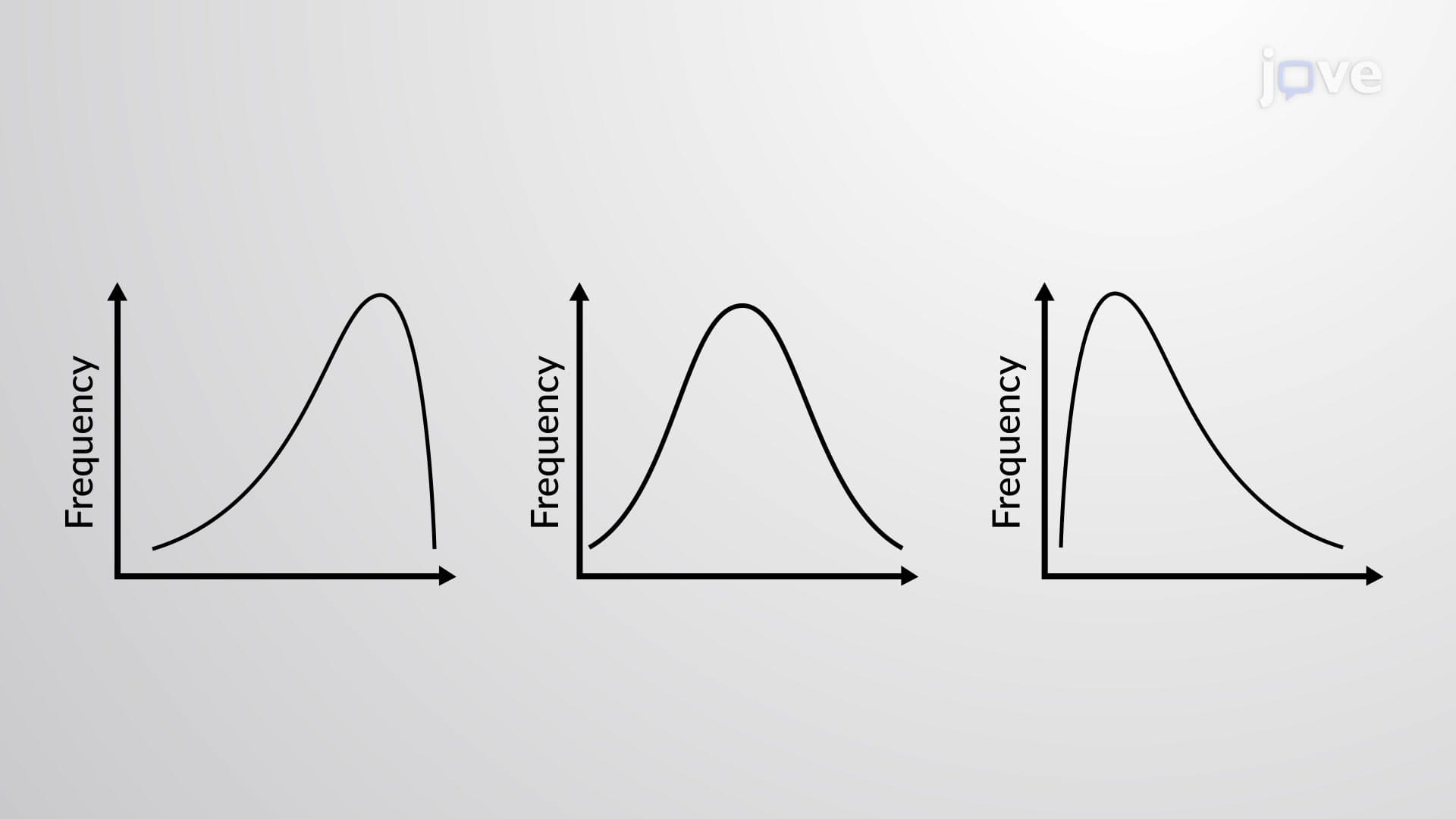
6. Skewness Analysis and Distribution Interpretation: Skewness indicates data asymmetry through tail direction and central tendency relationships. Normal distribution shows mean, median, and mode at identical positions. Positive skewness (right tail) occurs with income data where few earn extremely high amounts. Negative skewness (left tail) appears in easy exam scores where most students perform well. Understanding skewness helps interpret investment returns, standardized test score distributions, and demographic data patterns in social sciences.