Loading subject page…


2,477 views


Video Summary: What are Linear Differential Equations
Why does a car's speed level off instead of increasing forever? The answer lies in linear differential equations, a foundational concept in calculus and physics. What are Linear Differential Equations? This concept explains how quantities like velocity change over time under competing forces, using real-world scenarios like a car engine fighting air resistance on a US highway. Watch the full video on JoVE Coach to master this concept with expert-led visuals and step-by-step explanations.
A linear differential equation is an equation involving an unknown function and its derivatives, where the unknown function and all its derivatives appear to the first power only, never squared, cubed, or inside a nonlinear function like a sine or exponential. The most approachable form is the first-order linear differential equation, written in standard form as:
dy/dx + P(x)·y = Q(x)
Here, P(x) and Q(x) are functions of x alone, y is the unknown function, and dy/dx is its first derivative. This structure is what makes the equation "linear", the variable y never multiplies itself or its own derivative. Understanding this distinction is critical for students in AP Calculus BC and college-level Ordinary Differential Equations (ODE) courses across the US.
A common early confusion involves separable equations, where you can algebraically move all y-terms to one side and all x-terms to the other, then integrate both sides independently. That approach is elegant, but it only works when the equation allows clean separation.
Many real-world equations do not cooperate that way. When a car accelerates against air resistance proportional to its speed, for example, Newton's Second Law produces a first-order linear ODE that cannot be cleanly separated. This is precisely where the integrating factor method becomes essential. Recognizing whether an equation is separable or requires an integrating factor is a testable skill on AP Calculus BC exams and college midterms nationwide.
The integrating factor (commonly written as μ, or "mu") is defined as:
μ(x) = e^(integral of P(x) dx)
You find P(x) from the standard form of the equation, integrate it, and exponentiate the result. Once you have μ(x), you multiply both sides of the differential equation by it. The key insight, and the reason this method works, is that the left-hand side of the equation then becomes the derivative of the product μ(x)·y. In plain terms:
d/dx [μ(x)·y] = μ(x)·Q(x)
Now both sides can be integrated directly. The left side simplifies to μ(x)·y, and integrating the right side gives the general solution. If an initial condition is provided (for example, a car starting from rest means speed = 0 at time = 0), you substitute that value to find the constant of integration and obtain the particular solution, the unique curve that fits both the equation and the given starting point.
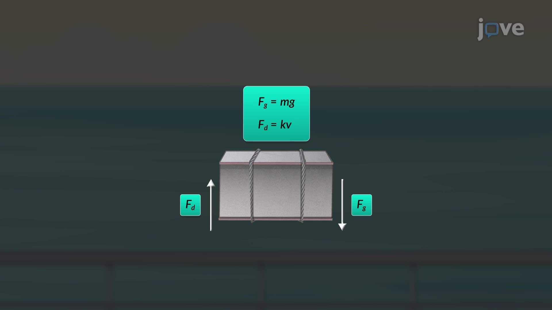
The car-and-air-resistance example is more than a textbook exercise. It models a genuine physical phenomenon: terminal velocity. When a parachutist jumps from an aircraft over a US military training facility or a skydiving center, the downward gravitational force competes with increasing air drag. The resulting first-order linear ODE predicts exactly when and at what speed the jumper stops accelerating.
The same mathematical structure appears in:
Students in AP Physics C, college Calculus II, and introductory ODE courses will encounter these applications repeatedly. Mastering the integrating factor method is not just an academic exercise, it is the gateway to modeling anything that changes continuously under competing influences.
Related Micro-courses