Vectors in Space

Vectors in Space Fundamentals builds essential 3D vectors calculus skills used across physics, engineering, and architecture. Powered by JoVE Coach, this micro-course covers vector components, the dot product and cross product, lines and planes in space, and quadric surfaces. Students apply these tools to real US engineering contexts — from suspension cables and solar panels to surveying instruments — developing the spatial reasoning required for college STEM success.

• Understand how vectors in space are represented using components, magnitude, and direction in three-dimensional coordinate systems
• Learn how to calculate the dot product and cross product of two vectors and interpret their geometric meanings
• Identify the angle between two vectors using the dot product formula and cosine relationships
• Apply vector equations to write parametric equations of a line and the scalar equation of a plane in 3D space
• Analyze real-world equilibrium problems involving cable tension, chandelier supports, and wind velocity using vector addition
• Explore cylindrical surfaces and quadric surfaces by examining traces and cross-sections in three-dimensional space
• Apply the cross product to calculate torque and area of a parallelogram in applied engineering scenarios
• Understand how the magnitude of a vector connects to the Pythagorean Theorem extended into three dimensions

1. Introduction to Vectors in Three-Dimensional Space A vector in 3D space is an arrow with both magnitude and direction, described numerically by components written in angle brackets — for example, ⟨3, 2, 1⟩. These components measure displacement along the x-, y-, and z-axes. When a vector originates from the origin, it is called a position vector. When it connects two distinct points A and B, its components equal the coordinate differences B minus A. The magnitude of a vector is its total length, calculated by extending the Pythagorean Theorem to three dimensions: the square root of the sum of the squared components. This foundational concept supports every subsequent topic in the course.

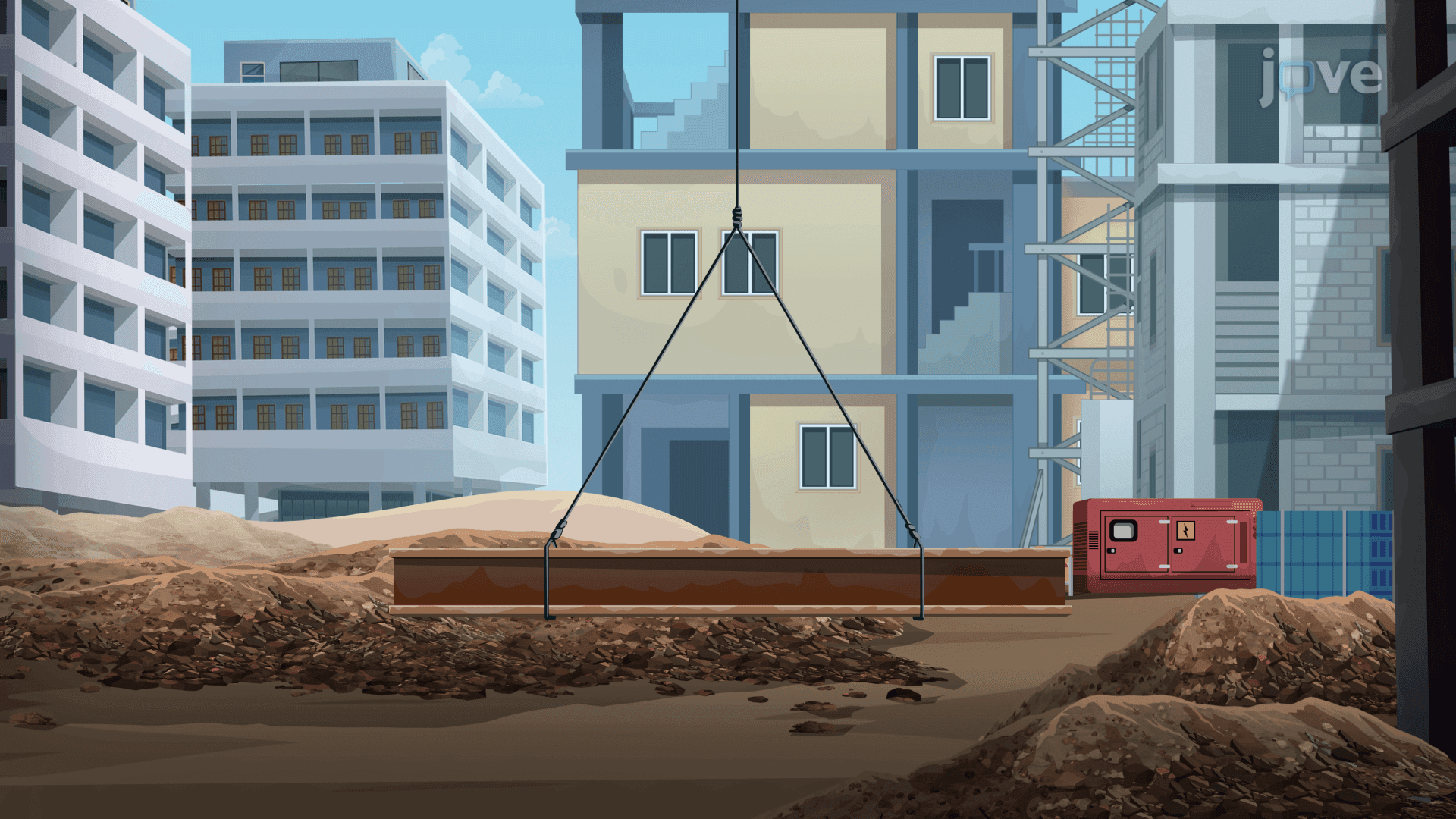
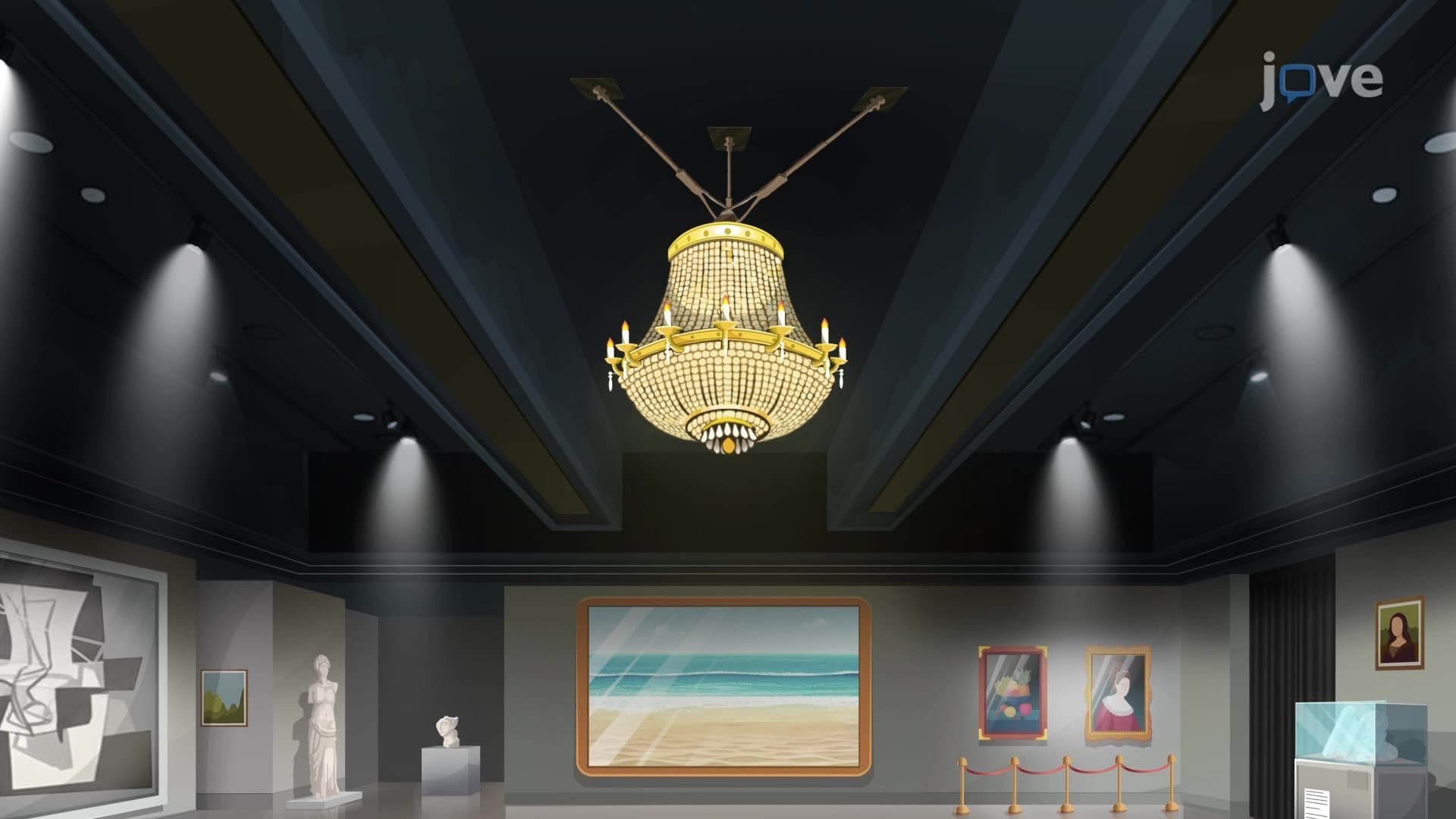
2. Vectors in Engineering Applications: Equilibrium and Forces Vectors become powerful problem-solving tools in engineering mechanics. A classic US construction scenario involves finding the tension in two symmetric cables supporting a steel beam. Each cable tension is resolved into horizontal and vertical components using unit vectors i and j. The condition of equilibrium — zero net force — sets up a system of equations. Balancing horizontal components confirms equal cable tensions; balancing vertical components determines the tension magnitude. Similarly, a three-cable chandelier problem in 3D requires unit vectors along each cable direction and a system of three equilibrium equations to solve for unknown tension scalars. These methods directly mirror techniques used in structural engineering practice.

3. Dot Product of Two Vectors The dot product takes two vectors and returns a single scalar value. Algebraically, it is computed by multiplying corresponding components and summing the results. Geometrically, the dot product equals the product of the two vectors' magnitudes multiplied by the cosine of the angle between them — making it the key tool for finding the angle between two vectors. A practical US application involves optimizing solar panel tilt: sunlight is modeled as a direction vector, and the panel's outward normal is another. Maximizing their dot product maximizes energy absorption. When the dot product equals zero, the vectors are perpendicular, and the panel receives no direct solar energy — a critical design threshold.

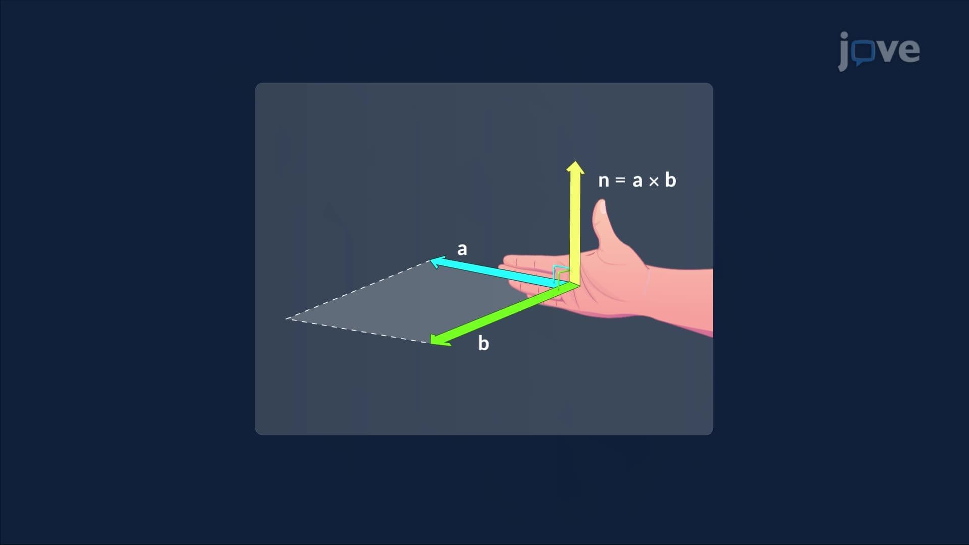
4. Cross Product and Its Geometric Interpretation The cross product of two non-parallel 3D vectors produces a new vector perpendicular to both. Its direction follows the Right-Hand Rule: point fingers along the first vector, curl them toward the second, and the thumb indicates the result. The geometric interpretation of the cross product is powerful — its magnitude equals the area of the parallelogram formed by the two original vectors, calculated using their magnitudes and the sine of the angle between them. This is maximized when vectors are perpendicular. A direct US engineering application is torque: when a wrench applies force to a bolt, torque is the cross product of the radius vector and the force vector, and it is maximized when force is applied at 90 degrees.

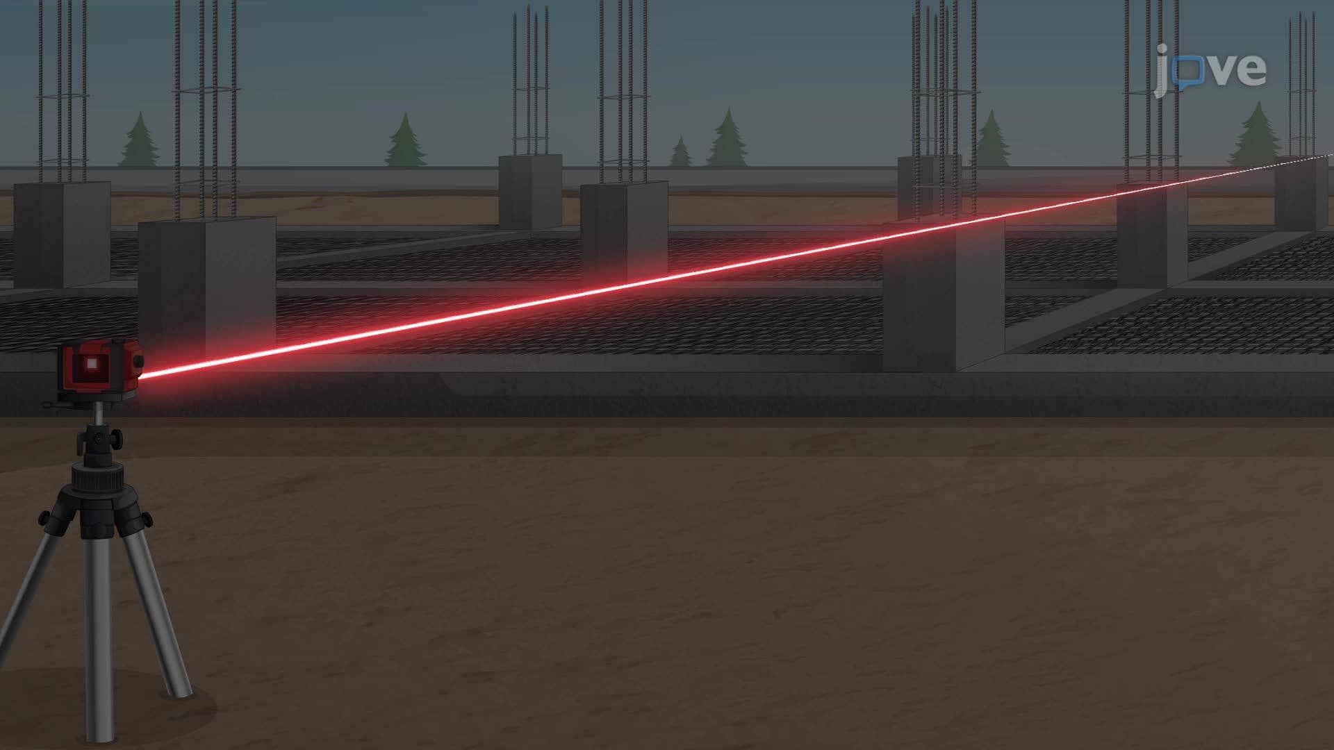
5. Parametric Equations of a Line in Space A line in 3D space is defined by a known point and a direction vector. Using vector addition, any point on the line is reached by starting at the fixed point and traveling a scalar multiple of the direction vector. This yields the vector equation of the line, which can be expanded into parametric equations — one for each coordinate. The scalar parameter traces the entire line: positive values extend in one direction from the starting point, negative values in the other. A practical US example is laser-based surveying: the surveying instrument emits a beam from a fixed location in a known direction, and the parametric form converts sensor data into precise spatial coordinates for construction alignment.

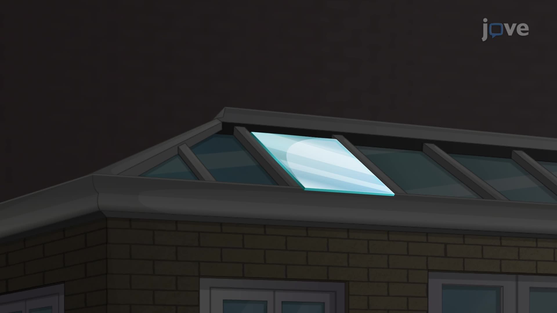
6. Equations of Planes in Space A plane in 3D space is uniquely determined by one point on the plane and a normal vector perpendicular to its surface. Any second point on the plane forms a vector with the fixed point; since this vector lies in the plane, it must be perpendicular to the normal — their dot product equals zero. This orthogonality condition produces the vector equation of the plane, which expands into the scalar equation using the normal vector's components and the fixed point's coordinates. A US architectural example is a sloped glass curtain wall panel: modeling the surface as a plane allows engineers to verify that mounting points satisfy the plane equation, ensuring structural alignment and precise installation.

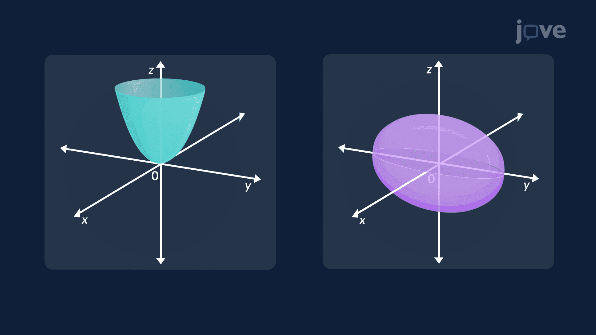
7. Cylinders and Quadric Surfaces in Three-Dimensional Space Cylindrical surfaces are formed when a 2D curve — called a profile curve — is extended infinitely along a straight-line direction, creating parallel rulings. In Cartesian equations, a missing variable reveals this extension: the equation y = x² describes a parabolic cylinder extending along the z-axis, used in tunnel and arch modeling. Quadric surfaces extend conic sections — ellipses, parabolas, hyperbolas — into 3D through second-degree equations in x, y, and z. Identifying a quadric surface requires analyzing its traces: cross-sections at constant values of each variable. When all traces are ellipses, the surface is an ellipsoid, widely used in US pressure vessel engineering because its curved geometry distributes internal pressure evenly across the surface.