Differentiation Rules

Differentiation Rules Fundamentals covers the essential differentiation rules that power modern calculus — from the power rule and product rule to implicit differentiation and hyperbolic functions. Guided by JoVE Coach, students explore how these basic differentiation rules connect to real US applications like engineering, biology, and physics. Mastering these rules of derivatives builds the analytical foundation required for AP Calculus, college-level STEM courses, and standardized exams.

• Understand the foundational differentiation rules — including the power, product, quotient, and chain rules — and recognize when each applies
• Learn how to differentiate trigonometric, logarithmic, exponential, and hyperbolic functions using systematic methods
• Apply implicit differentiation to curves and equations where dependent variables cannot be isolated, such as circles and ellipses
• Analyze rates of change in real-world contexts, including exponential population growth, related rates in expanding balloons, and velocity-acceleration problems
• Identify higher-order derivatives, including second derivatives of implicitly defined functions, and interpret their geometric meaning (concavity)
• Explore logarithmic differentiation as a technique for handling functions with variable bases and exponents
• Apply linearization and linear approximation to estimate function values near reference points in engineering and navigation contexts
• Understand inverse trigonometric and inverse hyperbolic function derivatives and their relevance to angle-tracking and structural design problems

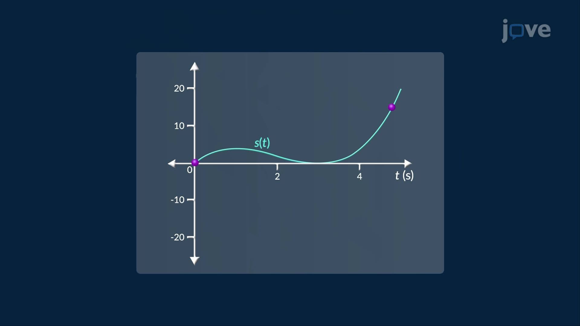
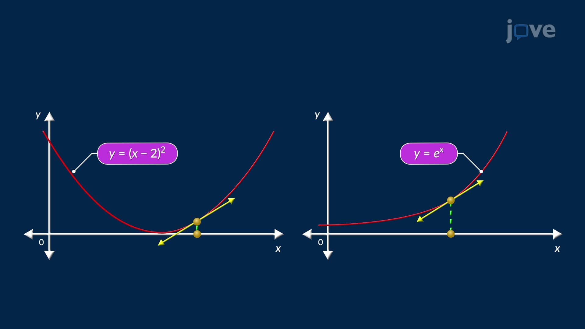
1. Derivatives of Simple Functions and the Power Rule The derivative measures the instantaneous rate of change of a function — visually, the slope of a tangent line to its curve. For constant functions, the derivative is always zero. For linear and polynomial functions, the power rule provides a systematic shortcut: multiply the coefficient by the exponent, then reduce the exponent by one. For example, the position of a car along a highway modeled as a polynomial yields velocity through differentiation. These foundational ideas underpin every advanced technique introduced throughout the course and appear directly on AP Calculus AB exams.

2. The Product Rule and the Quotient Rule When two functions are multiplied together, the product rule states that the derivative equals the first function times the derivative of the second, plus the second function times the derivative of the first. A useful analogy is a resizing rectangle: its area changes based on both dimensions shifting simultaneously. The quotient rule handles ratios of two functions — for example, a changing volume-to-drainage-rate ratio in a water tank. It equals the denominator times the numerator's derivative minus the numerator times the denominator's derivative, all divided by the denominator squared. Knowing when to apply the quotient rule versus the product rule is a common AP Calculus exam challenge.

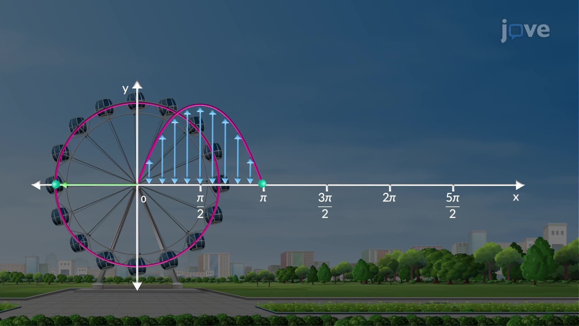
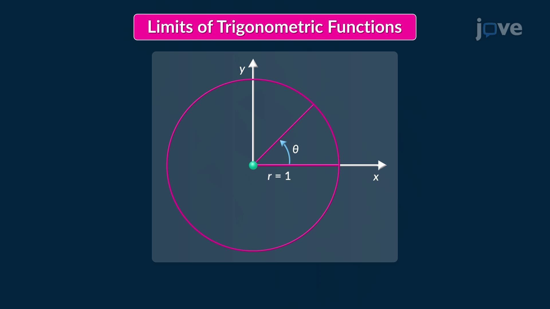
3. Derivatives of Trigonometric Functions and Their Limits Using the limit definition of a derivative and key trigonometric identities, the derivatives of sine, cosine, and tangent can be derived precisely. The derivative of sin(x) is cos(x); the derivative of cos(x) is −sin(x); and the derivative of tan(x) is sec²(x). Underlying these results is the fundamental trigonometric limit: as θ approaches zero, sin(θ)/θ approaches 1. This limit is proven geometrically using a unit circle. These derivatives are essential for modeling cyclical, oscillating phenomena — such as Ferris wheel height over time — and appear frequently in AP Calculus and college physics coursework.

4. The Chain Rule The chain rule differentiates composite functions — functions built by plugging one function into another. It states that the derivative of a composite equals the derivative of the outer function (evaluated at the inner function) multiplied by the derivative of the inner function. A three-gear mechanical system illustrates this perfectly: changes in the first gear's rotation propagate through intermediate gears to affect the last. In practice, the chain rule applies when differentiating expressions like sin(x²) or e^(3x). Understanding how to apply the chain rule is a critical skill tested on both AP Calculus AB and BC exams.

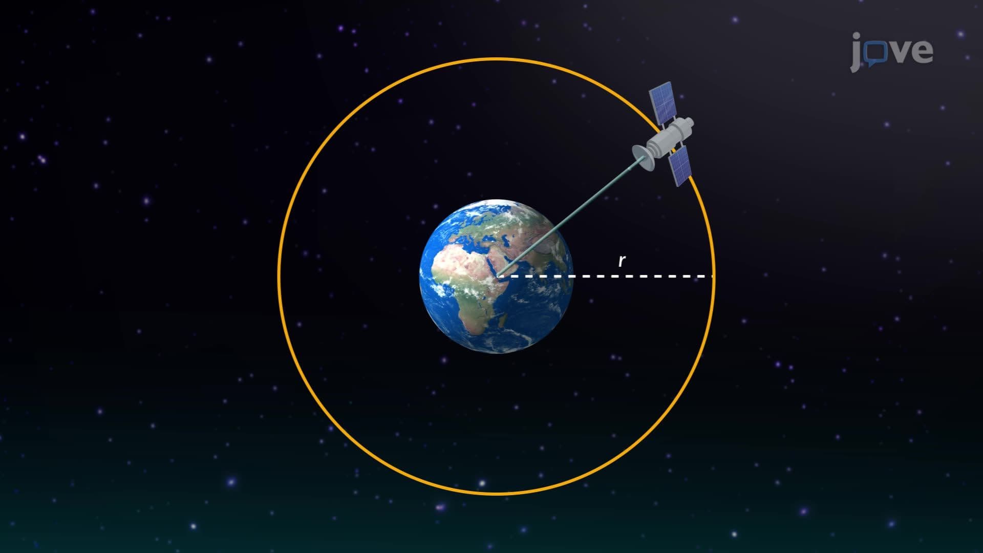
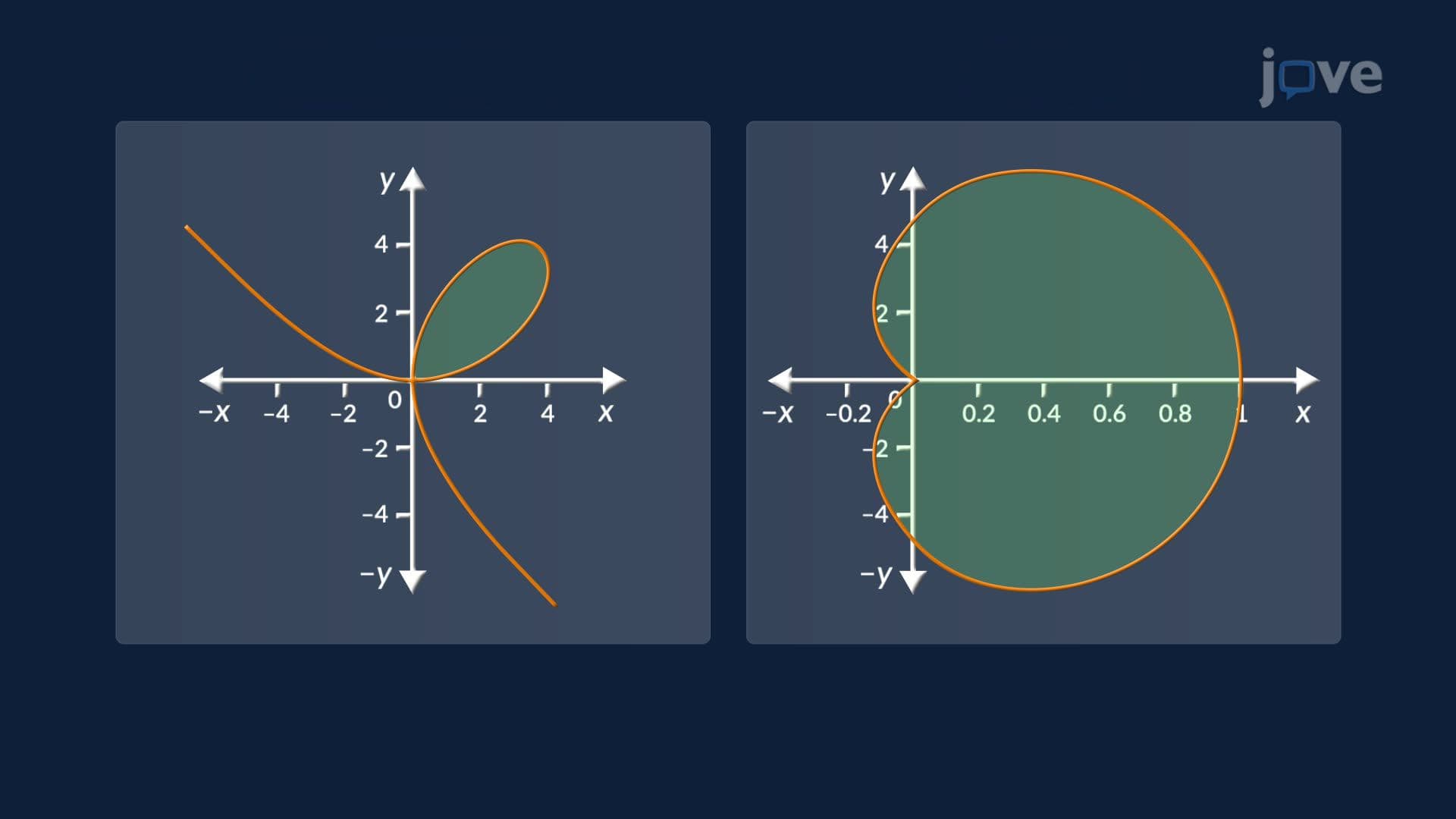
5. Implicit Differentiation and Higher-Order Derivatives Some equations — like those describing circular satellite orbits or elliptical bridge arches — cannot easily isolate one variable. Implicit differentiation differentiates both sides of the equation with respect to x, applying the chain rule wherever y appears, then solving for dy/dx algebraically. The second derivative requires differentiating dy/dx again using the quotient rule, then substituting the first derivative back in. A positive second derivative indicates concave-up curvature; a negative one indicates concave-down. For structural engineers analyzing arched bridges, these curvature insights directly inform stability assessments — making this topic relevant far beyond the classroom.

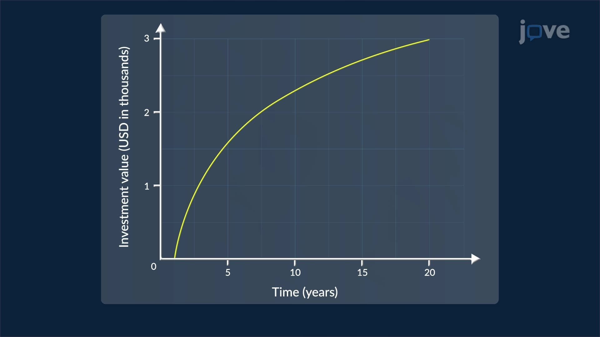
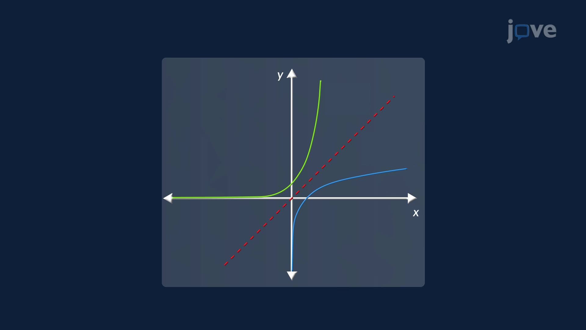
6. Logarithmic Functions and Logarithmic Differentiation The derivative of a logarithmic function with base b is 1/(x · ln b). When the base is e, this simplifies to 1/x, the derivative of the natural logarithm. This reciprocal relationship models diminishing returns — in finance, early investments grow faster, and the rate of return decreases over time. Logarithmic differentiation is a powerful technique for differentiating functions where both the base and the exponent contain variables, such as those describing stress-strain relationships in tire rubber. By taking the natural log of both sides first, the expression becomes more manageable before standard rules are applied.

7. The Number e, Exponential Growth, and Related Rates The constant e ≈ 2.718 emerges naturally from the derivative of the natural logarithm and from limits involving compounding interest. Exponential functions model bacterial population growth, where the rate of growth at any instant equals the growth constant multiplied by the current population. Related rates extend this thinking to situations where multiple changing quantities are linked — such as the radius and volume of an inflating hot air balloon. Differentiating the volume formula with respect to time connects how fast the volume changes to how fast the radius expands, a calculation critical for ensuring the balloon fabric does not exceed its rupture limit.

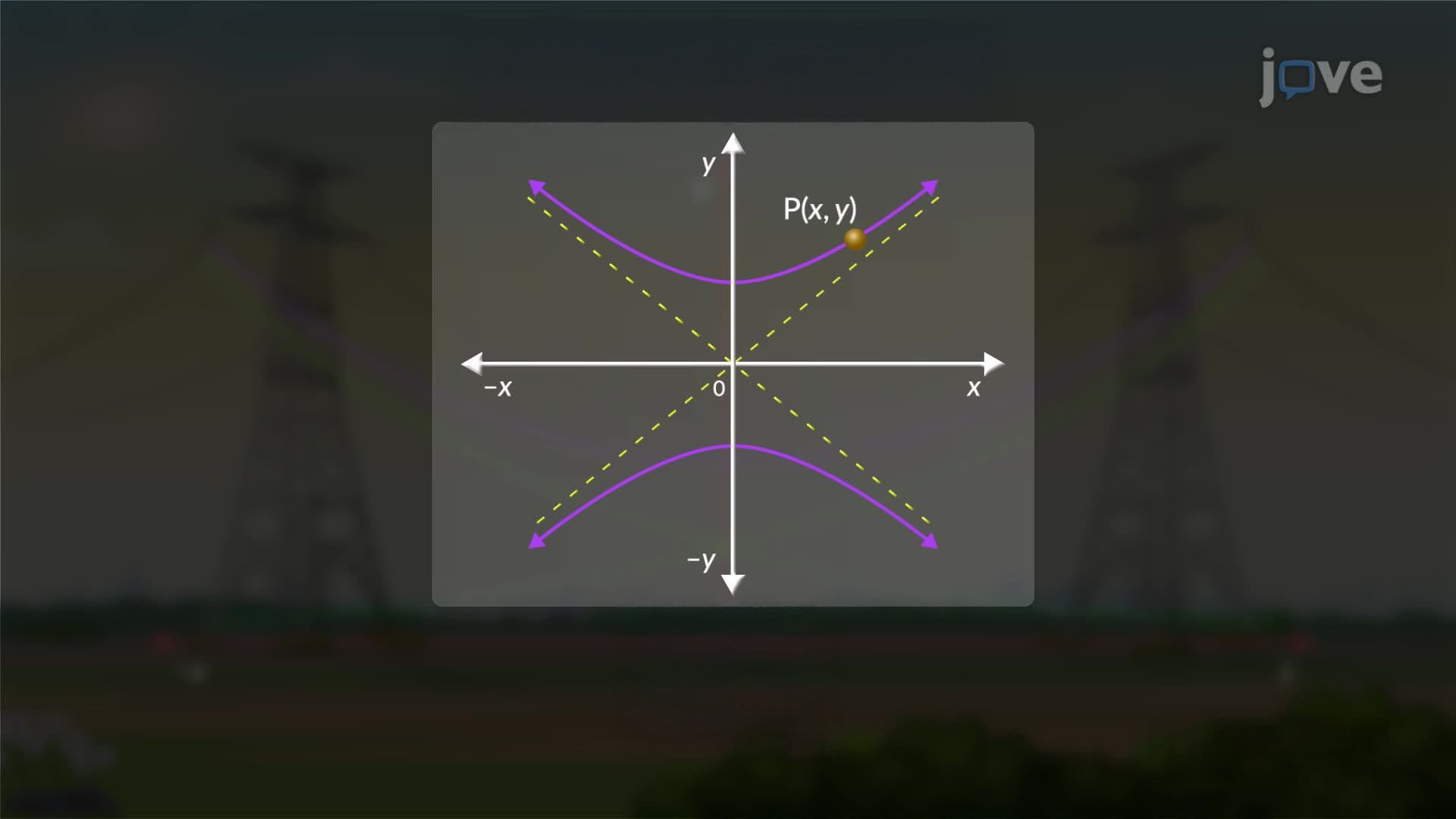
8. Inverse Trigonometric and Inverse Hyperbolic Functions The derivative of arcsin(x) is 1/√(1 − x²), derived by applying implicit differentiation and the Pythagorean identity. Similar techniques yield derivatives for arccos and arctan. These results have direct engineering applications — for example, radar systems tracking aircraft use the sensitivity of angle measurements to small position changes. Hyperbolic functions (sinh, cosh, tanh) and their inverses describe the shape of suspension bridge cables (catenaries) and other physical structures. The derivative of inverse hyperbolic cosine describes how horizontal cable position changes with vertical position, information structural engineers use to calculate cable tension and arch design.

9. Linearization, Approximation, and Rates of Change Linearization replaces a complex nonlinear function with a simpler tangent-line approximation near a specific reference point. The linear approximation formula combines the function's value and its derivative at the reference point to estimate nearby outputs — for example, approximating √4.1 using the known value and slope at x = 4. Drones use a similar method: altitude is estimated from air pressure readings using a linearized version of an exponential decay formula, accurate only for small pressure deviations. Related rates problems — where multiple variables change simultaneously — require differentiating a shared equation with respect to time, using the chain rule to connect all rates of change.