Application of Techniques of Integration

Techniques of integration form the backbone of solving real-world engineering, physics, and economics problems. This micro-course, supported by JoVE Coach, explores applications of integration techniques across arc length, surface area, hydrostatic pressure, center of mass, probability, and more. From designing roller coasters to modeling blood flow and consumer surplus, students discover how integration methods transform complex physical scenarios into precise, computable solutions.

• Understand how the arc length formula is derived using Riemann sums and definite integrals to measure curved distances along smooth paths
• Learn how surfaces of revolution are generated and how integration calculates their exact surface area for engineering applications
• Apply integration methods to compute hydrostatic force on submerged vertical surfaces, such as dam walls and underwater structures
• Identify how centers of mass and centroids are determined for continuous systems like thin rods and plane regions using moment integrals
• Explore Pappus's Theorem to find volumes of solids of revolution without directly applying disk or shell integration techniques
• Analyze how definite integrals quantify consumer surplus, blood flow via Poiseuille's Law, and probability using density functions
• Apply the arc length function and its rate of change using the Fundamental Theorem of Calculus to real-world measurement problems
• Understand normal distributions and probability density functions, connecting continuous data to area under a curve

1. Arc Length of a Curve Arc length measures the actual distance along a curved path rather than the straight-line distance between two points. The derivation begins by dividing a curve into small segments and approximating each with a straight line using the distance formula. Applying the Mean Value Theorem introduces the derivative into each segment's length. As the number of segments increases without bound, the approximation becomes a definite integral. The standard arc length formula integrates the square root of one plus the square of the derivative over a given interval. In practice, this applies to designing roller coaster tracks, mapping highway curves, and calculating the length of suspension bridge cables across US infrastructure projects.

2. Arc Length Function and Rate of Change The arc length function extends the arc length concept by treating the endpoint as a variable, producing a function that tracks cumulative distance from a fixed starting point. A dummy integration variable is used so the upper limit can vary freely. The integrand, the square root of one plus the squared derivative, is always at least one, growing larger as the curve steepens. Differentiating the arc length function using the Fundamental Theorem of Calculus recovers this integrand, revealing that the rate of change of arc length depends directly on slope. This is directly useful in surveying and road barrier installation along winding US mountain highways.

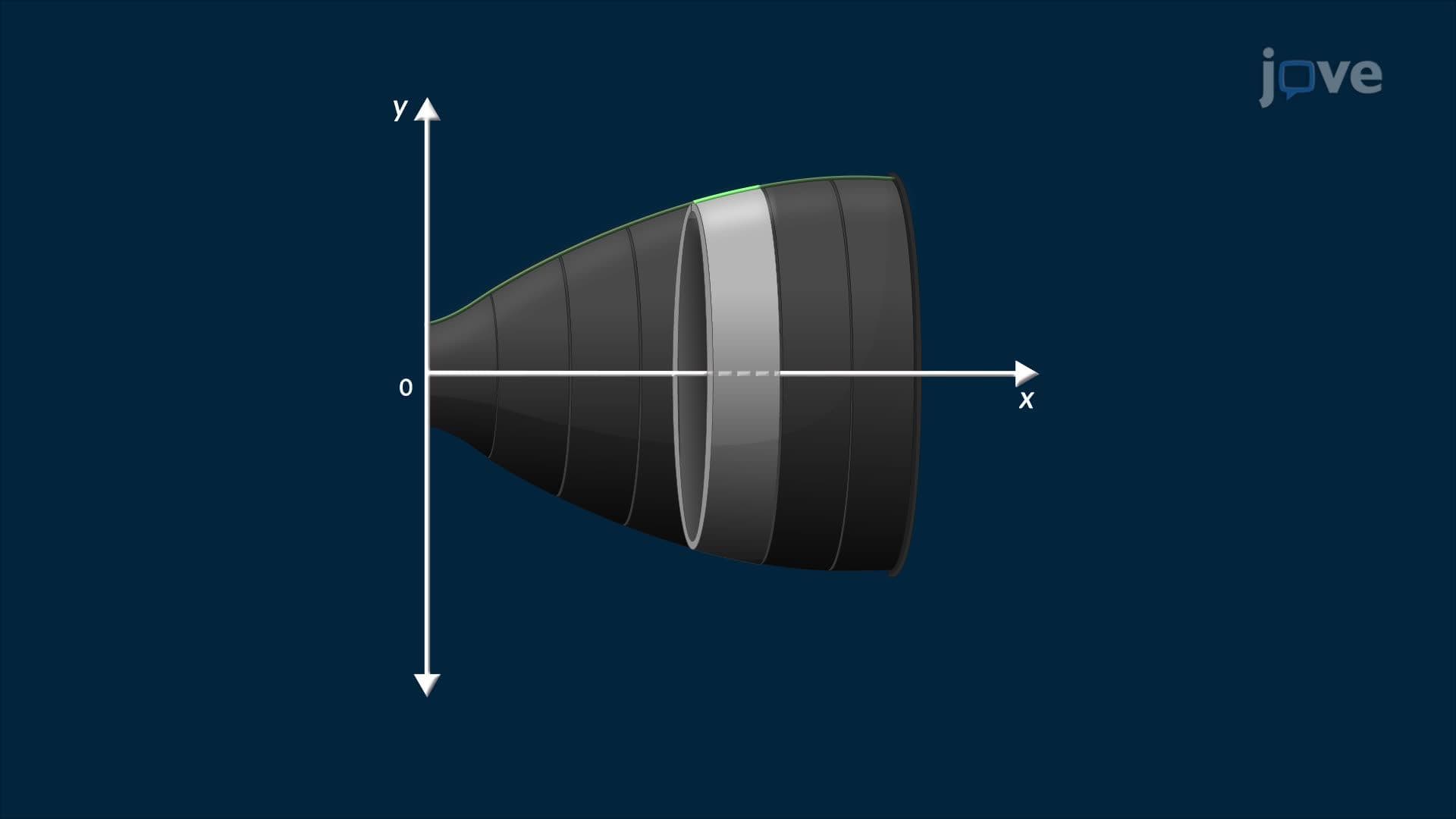
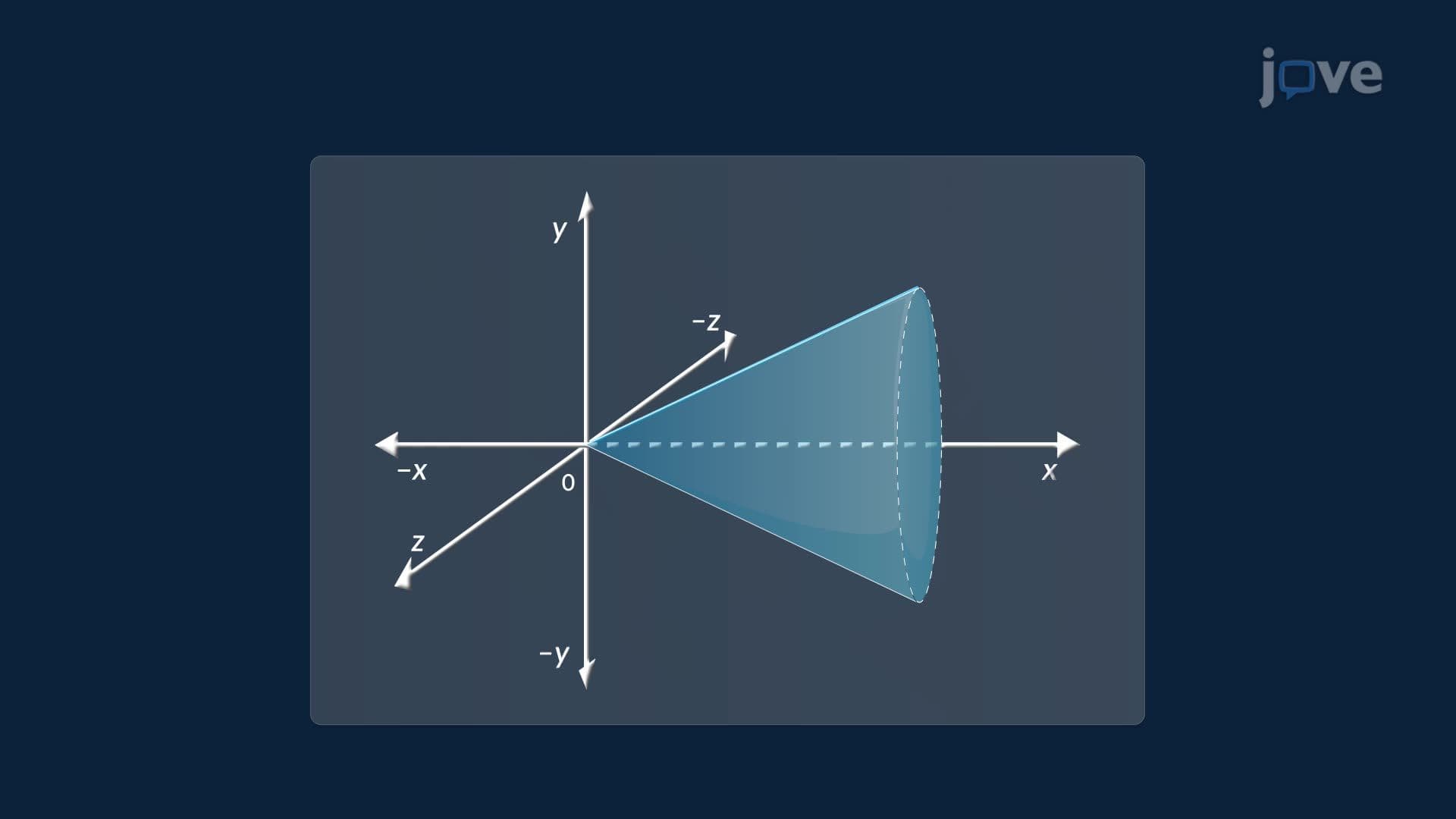
3. Surface Area of Revolution When a curve is rotated around an axis, it sweeps out a three-dimensional surface called a surface of revolution. To find its exact area, the curve is divided into small segments, each approximated by a line segment. Revolving each segment creates a narrow frustum, a conical band, whose surface area equals the average radius times the slant height times 2π. The slant height incorporates the arc length element, accounting for the curve's steepness. As segments shrink to zero width, the Riemann sum becomes a definite integral. Engineers use this to calculate the precise amount of heat-resistant coating needed for rocket engine nozzles and aerospace components manufactured in the US.

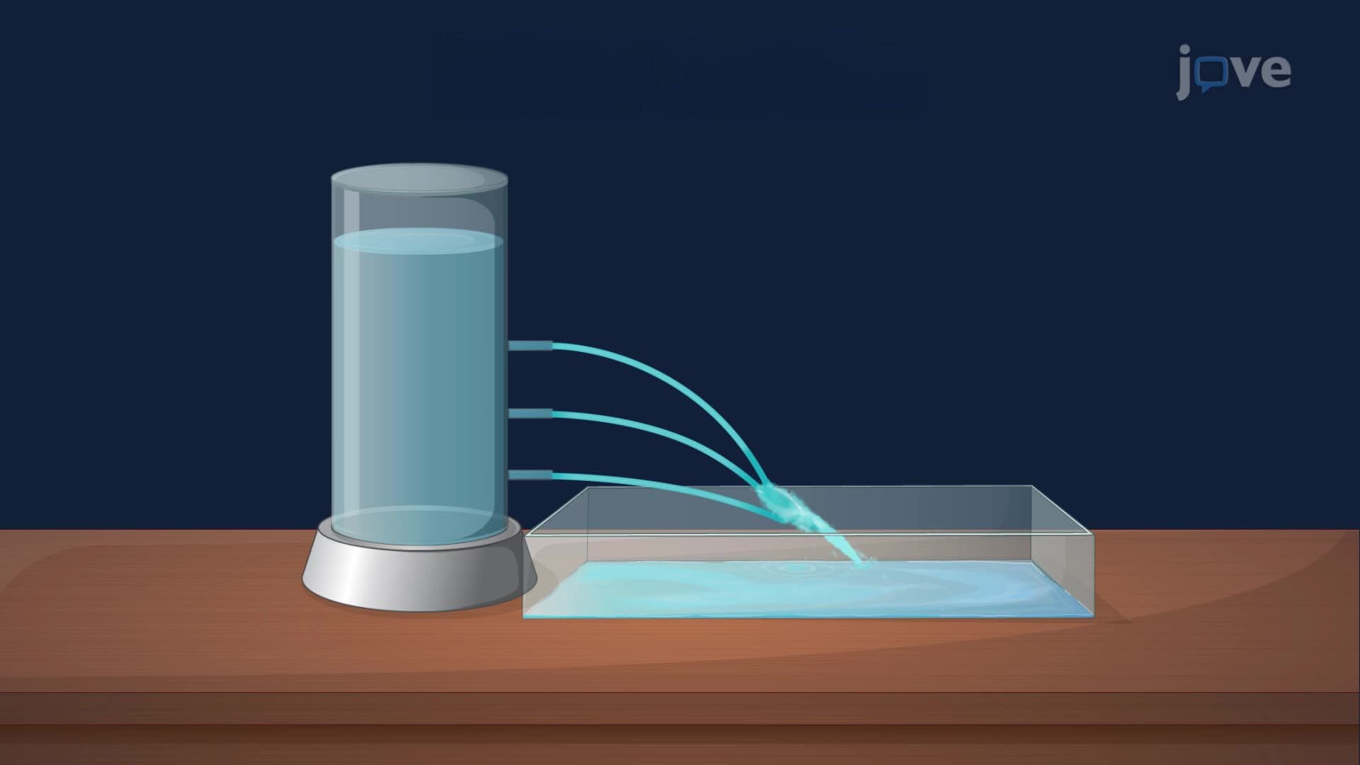
4. Hydrostatic Pressure and Force Hydrostatic pressure is the force per unit area exerted by a fluid at rest and increases linearly with depth. For a horizontal surface at constant depth, pressure is uniform. However, a vertical surface, like the face of the Hoover Dam, experiences varying pressure at every depth level. To calculate total hydrostatic force, the submerged surface is sliced into thin horizontal strips. Each strip experiences a nearly constant pressure equal to the fluid's weight density multiplied by its depth. Multiplying pressure by strip area and summing over all strips produces a Riemann sum. As strip thickness approaches zero, this sum converges to a definite integral that gives the exact total force, critical for safe dam and retaining wall design.

5. Center of Mass and Pappus's Theorem The center of mass is the point where a system's total mass can be considered concentrated for rotational analysis. For discrete masses on a beam, it equals the sum of moments (mass × position) divided by total mass. For continuous objects like a thin rod with variable density, this becomes an integral of the density-weighted position divided by total mass. Pappus's Theorem extends this to three dimensions: rotating a plane region around an external axis generates a solid whose volume equals the region's area multiplied by the circumference of the path traced by its centroid. This elegant result calculates volumes of toroidal fuel tanks, used in aerospace and automotive industries, without setting up complex revolution integrals directly.

6. Consumer Surplus and Economic Applications Consumer surplus measures the economic benefit consumers receive when they pay less than they were willing to pay. It is visualized as the area between a product's demand curve, which graphs maximum willingness to pay against quantity, and the actual constant market price line. To compute this area, the quantity interval is divided into subintervals. The difference between the demand curve value and the market price over each subinterval, multiplied by subinterval width, gives a partial surplus estimate. Summing all estimates forms a Riemann sum that converges to a definite integral. This integral precisely quantifies total consumer surplus, a key metric in US economic policy analysis and market efficiency studies taught in AP Microeconomics and college economics.

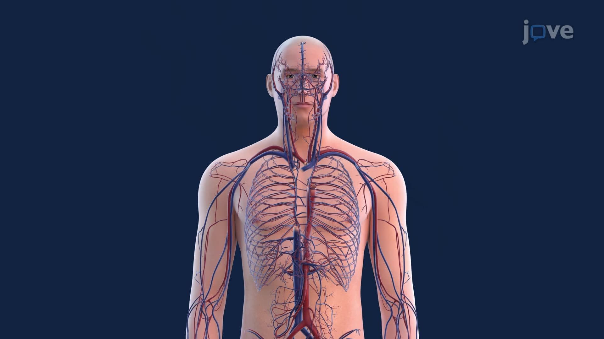
7. Blood Flow and Poiseuille's Law Blood flow through a vessel follows laminar flow principles, where velocity is highest at the center and decreases toward the vessel wall. To find the total volumetric flow rate, the circular cross-section is divided into thin concentric rings. Each ring's area equals its circumference multiplied by its small radial thickness. The flow through each ring is approximated by multiplying area by velocity at that radius. Summing ring flows gives a Riemann sum that, in the limit, becomes a definite integral. Substituting the laminar velocity function, which depends on pressure difference, viscosity, and vessel length, and integrating yields Poiseuille's Law: flow scales with the fourth power of vessel radius. This explains why arterial narrowing dramatically reduces blood flow, a critical concept for MCAT preparation.

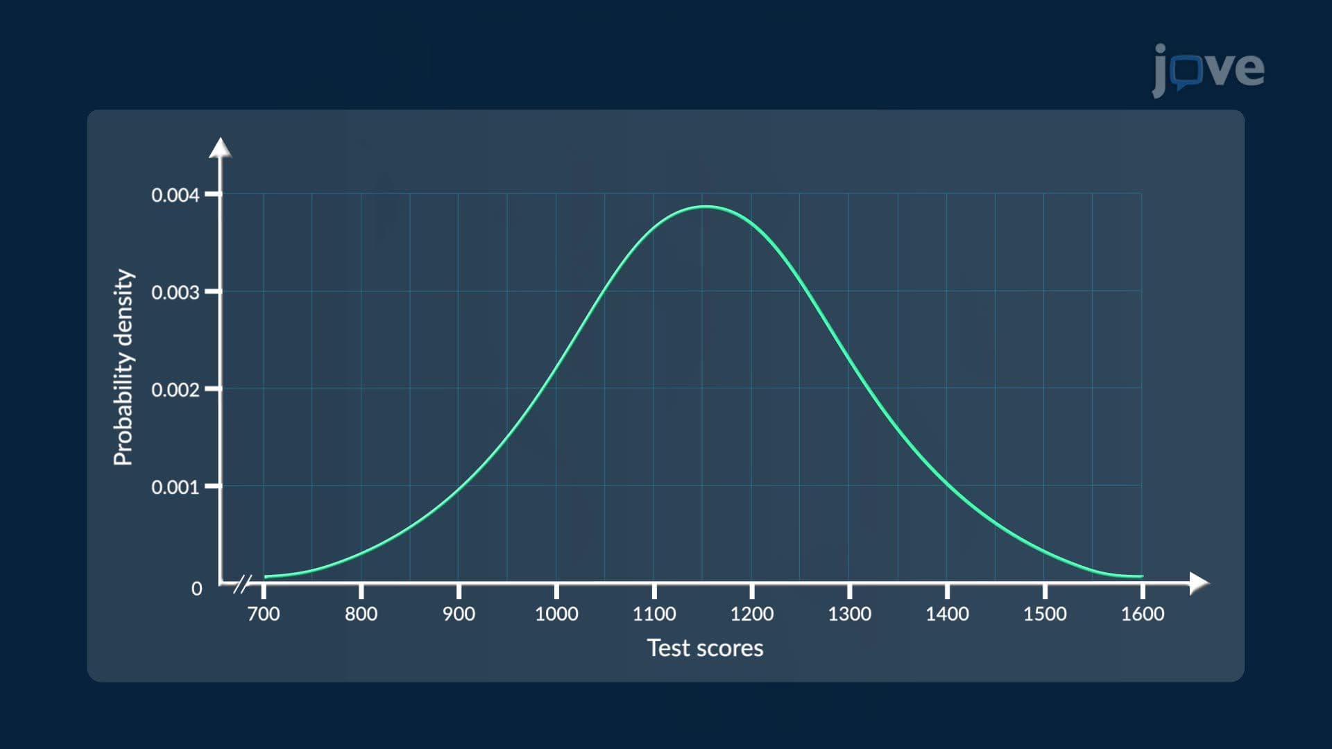
8. Normal Distributions and Probability Density Functions A probability density function (PDF) is a non-negative continuous function where the total area under the curve equals exactly one, representing 100% probability. The normal distribution, characterized by its symmetric bell shape, is defined by two parameters: the mean (center of the distribution) and the standard deviation (measure of spread). The probability that a continuous random variable falls within any specific interval equals the definite integral of the PDF over that interval. Integrating over a single point yields zero area, meaning exact values have zero probability. Normal distributions model standardized test scores, patient measurements in clinical trials, and manufacturing tolerances, making them foundational for AP Statistics, college probability courses, and MCAT data interpretation sections.