Loading video…

 11 Concepts
 3.3K views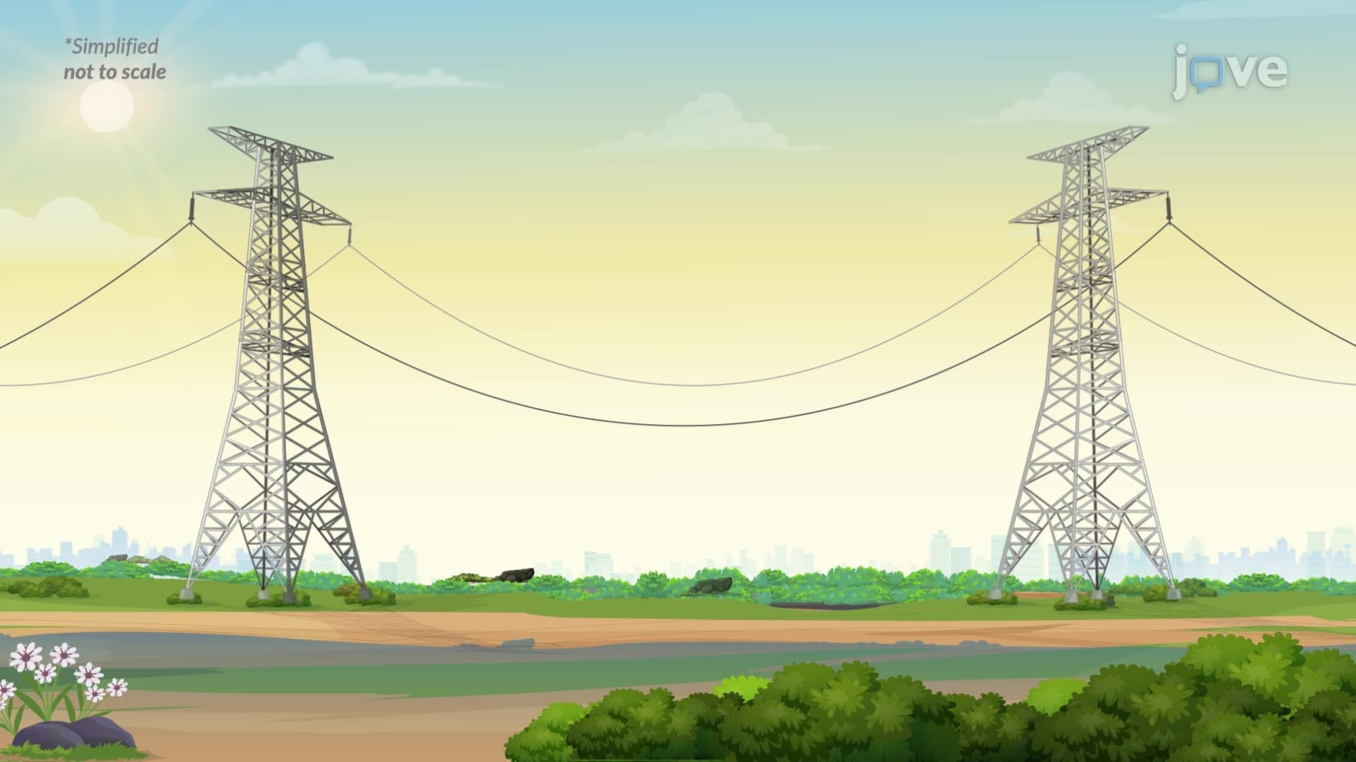

Video Summary: Problem Solving in Arc Length of a Curve
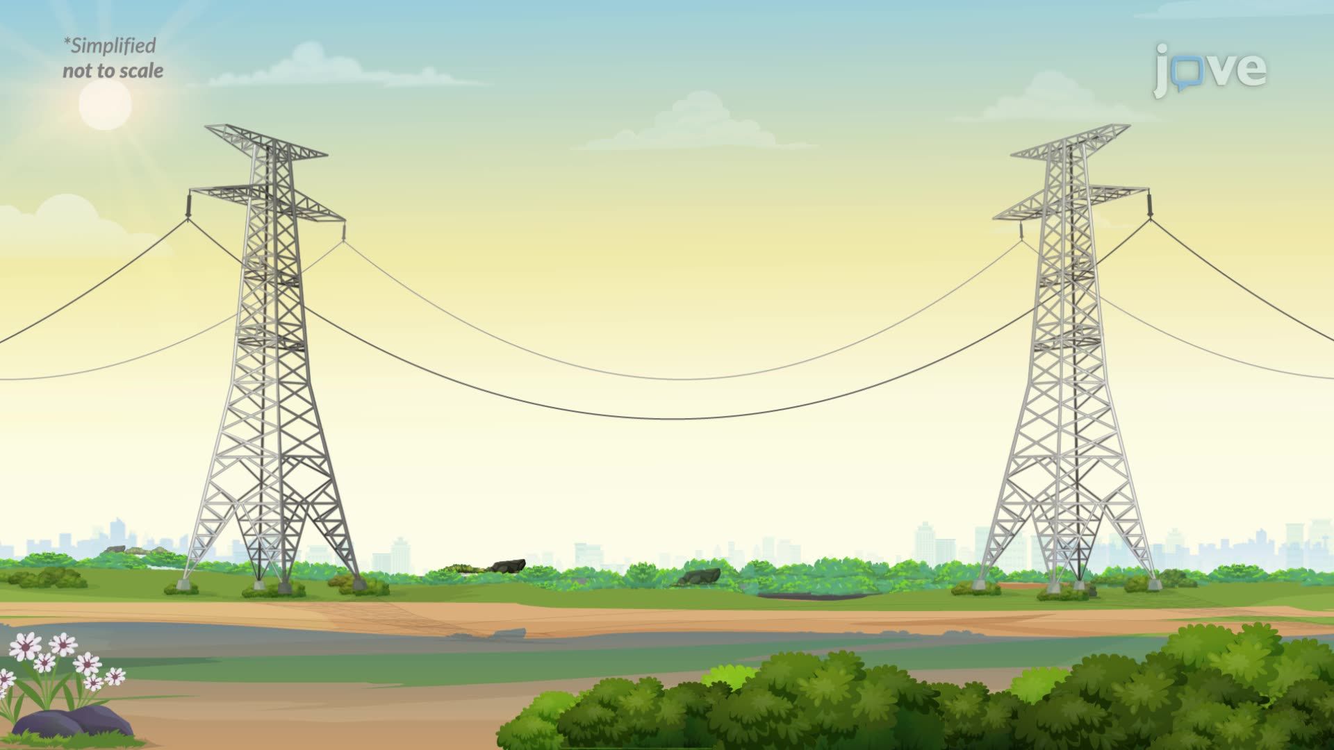
Did you know the power lines stretching between utility towers across American highways are actually longer than the distance they span? Problem solving in arc length of a curve reveals exactly how engineers calculate this hidden extra length. Using a catenary curve modeled by the hyperbolic cosine function, a 40-meter span with a 10-meter sag requires roughly 47 meters of cable. Watch the full video on JoVE Coach to master this concept with expert-led visuals and step-by-step explanations.
Arc length is one of the most satisfying applications of calculus because it turns an abstract integral into a real, measurable distance. Whether you are designing a suspension bridge cable in California or routing electrical transmission lines across Texas, the mathematics behind arc length gives engineers a precise answer to a deceptively simple question: how long is that curve?
The arc length of a smooth curve y = f(x) from x = a to x = b is given by the integral of the square root of (1 + (dy/dx)²) with respect to x. This formula comes directly from the Pythagorean theorem applied to infinitely small segments of the curve. Each tiny piece of the curve can be approximated as the hypotenuse of a right triangle with legs dx and dy. Integrating these infinitesimal lengths across the entire interval gives the total arc length. In practice, this integral is often difficult to evaluate by hand, which is why choosing the right function model, one whose derivative produces a clean expression under the square root, matters enormously.
A catenary is the shape a perfectly flexible, uniform cable naturally forms when suspended from two endpoints under gravity alone. It looks like a parabola but behaves differently mathematically. The catenary is described by y = a · cosh(x/a), where cosh is the hyperbolic cosine function and *a* is a parameter determined by the ratio of horizontal tension to the cable's weight per meter. This curve appears throughout American infrastructure, from the Gateway Arch in St. Louis (which is an inverted catenary) to high-voltage transmission lines spanning rural landscapes. For the power line problem, with a = 20 meters and a horizontal span of 40 meters (from x = −20 to x = 20), this model produces a physically accurate prediction of cable length.
What makes the catenary especially elegant in arc length problems is how its derivative behaves. The derivative of a · cosh(x/a) with respect to x is sinh(x/a), the hyperbolic sine. When you substitute this into the arc length formula, the expression under the square root becomes 1 + sinh²(x/a). Here is where a powerful identity kicks in: cosh²(x) − sinh²(x) = 1 means that 1 + sinh²(x) = cosh²(x). The square root disappears entirely, leaving a clean integral of cosh(x/a). Since the integral of cosh(x/a) is a · sinh(x/a), evaluation at the limits x = 20 and x = −20 is straightforward. This elegance is not accidental, it reflects why engineers specifically use the catenary model rather than, say, a parabola, when precision matters.
Arc length problems appear prominently on the AP Calculus BC exam and in Calculus II courses at US colleges and universities. Students are expected to set up the arc length integral correctly, simplify using algebraic or trigonometric identities, and evaluate, either exactly or using numerical methods like Simpson's Rule when a closed form is unavailable. Related techniques tested in the same units include integration by parts, trigonometric integrals, partial fractions, and improper integrals. Understanding how to apply integration to find length, and by extension, surface area and volume, builds the conceptual fluency that these courses and exams demand. Mastery of arc length also prepares students for physics and engineering coursework where these calculations appear in the analysis of projectile paths, satellite orbits, and structural load distributions.
Related Micro-courses