Loading video…


 11 Concepts
 3.3K views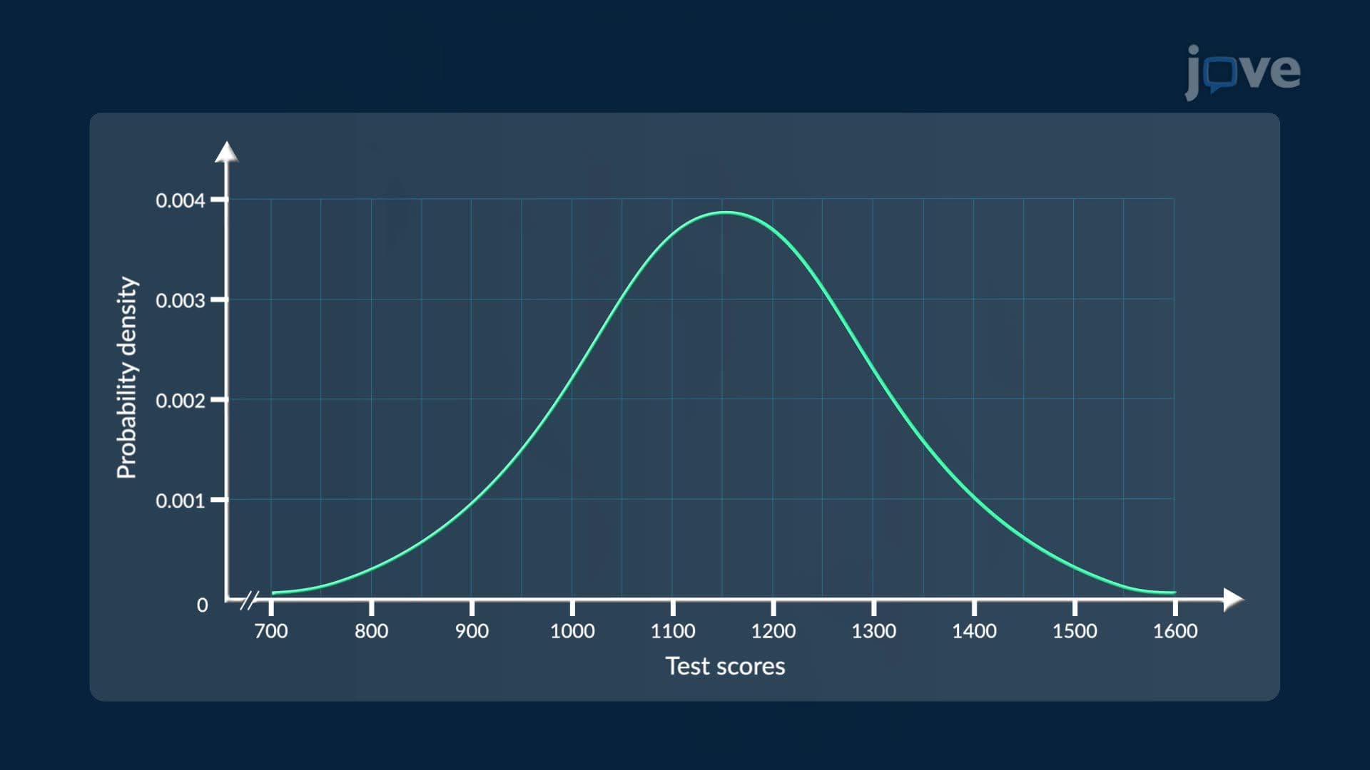

Video Summary: What are Normal Distributions
Did you know SAT math scores across millions of students form a nearly perfect bell-shaped curve? That's the power of normal distributions. Understanding normal distributions basics reveals how data clusters around a mean, with spread measured by standard deviation. The area under the curve always equals 1, representing 100% probability. Watch the full video on JoVE Coach to master this concept with expert-led visuals and step-by-step explanations.
Normal distributions describe a symmetric, bell-shaped pattern that appears naturally across countless datasets, from student test scores to human heights to manufacturing tolerances. At its core, a normal distribution is a continuous probability distribution fully defined by just two parameters: the mean (μ) and the standard deviation (σ). Once you understand these two values, you can describe, predict, and compare data with remarkable precision.
The intuition behind a normal distribution starts with a simple histogram. Imagine plotting ACT scores for 50,000 students, dividing scores into ranges (bins) and counting how many students fall in each. As you collect more data and narrow each bin, the jagged bars begin to smooth. Converting frequency counts into probability density (occurrences divided by total count and bin width) shifts the vertical axis from raw counts to proportional likelihood. As bins approach zero width, the histogram transforms into a smooth, continuous curve, the normal distribution.
The shape of the normal curve is governed by its probability density function (PDF):
f(x) = (1 / (σ × √(2π))) × e^(−(x − μ)² / (2σ²))
While this may look intimidating, its logic is straightforward. The expression centers the curve at the mean (μ) and the standard deviation (σ) stretches or compresses its width. The exponential term ensures the curve falls off symmetrically on both sides. A small σ produces a tall, narrow peak, scores are tightly packed near the mean. A large σ produces a wide, flat curve, scores are widely scattered. This is essential knowledge for AP Statistics and college-level probability courses.
One of the most powerful features of normal distributions is that area equals probability. The area under the curve between any two values on the x-axis represents the probability that a randomly selected data point falls within that range. For example, in a normal distribution of SAT scores with a mean of 1060 and a standard deviation of 217, you can calculate the probability that a student scored between 843 and 1277, which corresponds to one standard deviation on either side of the mean, covering approximately 68% of all test-takers.
When the PDF is integrated across all possible values, from negative infinity to positive infinity, the total area equals exactly 1, or 100%. This is a fundamental requirement for any valid probability distribution: all possible outcomes must collectively account for certainty. This property directly connects normal distributions to concepts like improper integrals and the broader real-world applications of integration techniques studied in calculus.
Normal distributions are everywhere in the United States' academic and professional landscape. The College Board designs the SAT and AP exams with the expectation that large-scale score distributions approximate normality. Medical researchers use normal distributions to define healthy ranges for lab values, a concept foundational to MCAT prep and clinical coursework. In manufacturing, quality control engineers use normal distributions to set tolerance thresholds. In psychology and education, standardized assessments like the IQ test are deliberately scaled to follow a normal distribution with a mean of 100 and a standard deviation of 15. Mastering this concept prepares students not just for exams, but for data-driven thinking across virtually every field.
Related Micro-courses