Differential Equations

Differential equations fundamentals form the mathematical backbone of science, engineering, and economics. This micro-course, supported by JoVE Coach, guides students from core definitions through real-world modeling — covering separable equations, linear first-order equations, integrating factors, and orthogonal trajectories. US applications include population dynamics, spring-mass systems, vehicle motion, and Newton's Law of Cooling, making abstract theory immediately practical.

• Understand what a differential equation is, how its order is determined, and why it differs from standard algebraic equations
• Identify separable differential equations and apply step-by-step integration techniques to find their general and particular solutions
• Learn how the integrating factor method works for solving first-order linear differential equations that cannot be separated
• Explore real-world modeling scenarios, including exponential population growth, logistic growth with carrying capacity, and Newton's Law of Cooling
• Analyze orthogonal trajectories and their geometric relationship to families of curves, with connections to electromagnetic field lines and equipotential surfaces
• Apply differential equations to physics-based problems, including spring-mass oscillators, falling objects with air resistance, and vehicles reaching terminal velocity
• Understand the difference between general solutions and particular solutions obtained through initial value conditions

1. What Is a Differential Equation? A differential equation is any equation that relates an unknown function to one or more of its derivatives. The order of the equation is set by the highest derivative it contains — first order involves only the first derivative, second order involves the second derivative, and so on. A classic US physics example is the spring-mass system: applying Hooke's Law and Newton's Second Law together produces a second-order differential equation in which the second derivative of displacement appears directly. Understanding this structure — identifying the unknown function, its derivatives, and the equation's order — is the essential first step in solving any differential equation problem.

2. Modeling with Differential Equations Differential equations translate real-world assumptions into mathematical language. Two foundational models illustrate this well. Exponential growth assumes a population increases at a rate proportional to its current size — a first-order ordinary differential equation with an exponential solution. The more realistic logistic growth model introduces a carrying capacity M, the maximum sustainable population size. Growth slows as the population approaches M and reverses if it overshoots. These models appear in AP Biology, AP Environmental Science, and MCAT prep, making them highly testable and practically significant for students pursuing US college entrance exams or health sciences programs.

3. Separable Differential Equations A separable equation is a first-order differential equation that can be algebraically rearranged so that all terms involving the dependent variable (typically y) are on one side and all terms involving the independent variable (typically x or t) are on the other. Once separated, both sides are integrated independently. Newton's Law of Cooling — where a hot object loses heat at a rate proportional to the temperature difference between the object and its surroundings — is a textbook example. The solution produces an exponential decay function. Finding a particular solution requires applying an initial condition, such as the starting temperature at time zero, to determine the integration constant.

4. Orthogonal Trajectories Two families of curves are called orthogonal trajectories if every curve from one family intersects every curve from the other at a perfect right angle (90°). To find orthogonal trajectories mathematically, the slope of the original family is found through differentiation, and then the negative reciprocal of that slope defines the perpendicular direction. Integrating this new differential equation produces the orthogonal family. A concrete example: parabolas of the form x = ky² have ellipses centered at the origin as their orthogonal trajectories. In physics, electric field lines and equipotential surfaces in electrostatics are real-world orthogonal trajectories, directly connecting this calculus concept to AP Physics and engineering coursework.

5. Linear First-Order Differential Equations and Integrating Factors Not all first-order differential equations are separable. A linear first-order differential equation has the standard form dy/dx + P(x)y = Q(x). The integrating factor method provides a reliable technique for solving these equations. The integrating factor μ(x) is calculated as e raised to the integral of P(x). Multiplying both sides of the equation by μ(x) transforms the left-hand side into the derivative of a product, making integration straightforward. A practical US example: a car driven by a constant engine force while experiencing air resistance proportional to speed follows this exact equation type. The solution predicts how the car accelerates quickly at first, then asymptotically approaches terminal velocity.

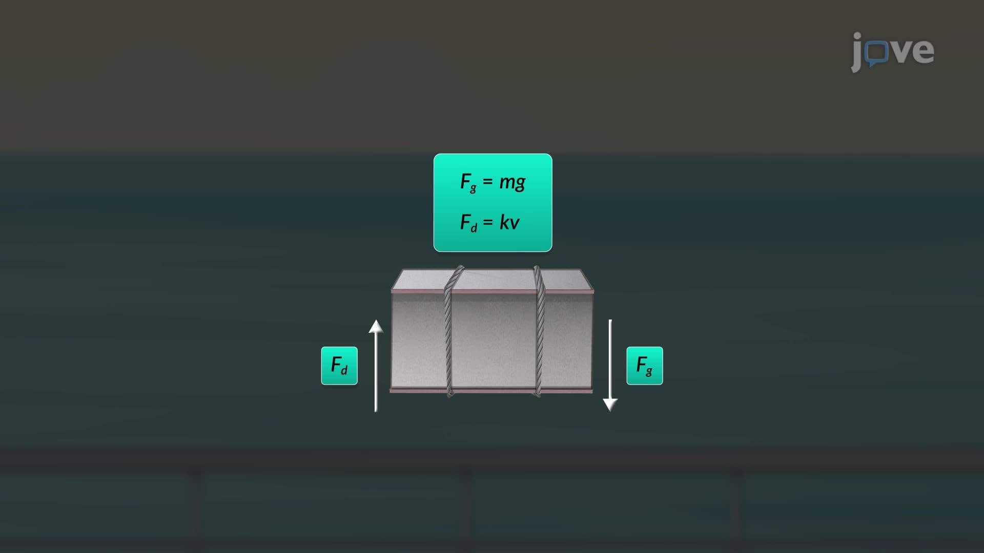
6. Solving Differential Equations: Initial Value Problems An initial value problem (IVP) pairs a differential equation with one or more specific conditions that anchor the solution to a particular scenario. General solutions contain arbitrary constants representing an entire family of curves; initial conditions reduce that family to a single, unique particular solution. The falling weight problem demonstrates this clearly: a 10 kg test weight dropped from rest with a drag constant of 2 N·s/m follows a separable differential equation. Applying the initial condition — velocity equals zero at time zero — determines the constant of integration, yielding an explicit equation for velocity over time and a predicted terminal velocity of 49 m/s.