Derivatives

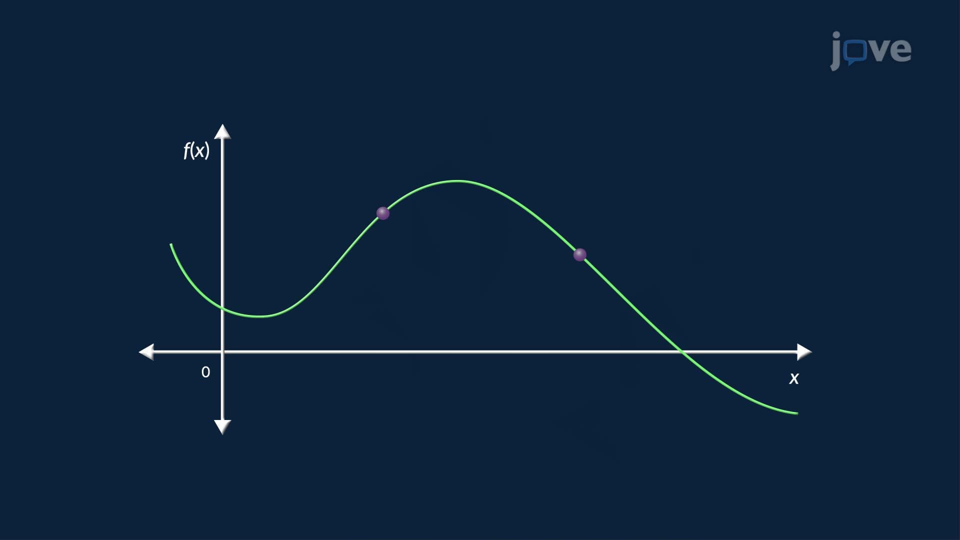
Derivatives fundamentals form the backbone of calculus, connecting abstract math to real-world change. This micro-course covers the limit definition of derivative, tangent and secant lines, rates of change, derivative functions, higher-order derivatives, and numerical estimation. From instantaneous velocity on a highway to acceleration in physics, JoVE Coach presents these concepts through clear, applied examples designed to build lasting conceptual understanding.

• Understand how secant lines approximate the slope of a curve and how their limit produces a tangent line
• Learn the limit definition of the derivative and apply it to compute derivatives algebraically
• Identify the difference between average rate of change and instantaneous rate of change using real-world contexts
• Explore how the derivative function assigns a slope value to every point in a function's domain
• Analyze higher-order derivatives — including velocity, acceleration, and jerk — as a hierarchy of rates of change
• Apply forward, backward, and central difference methods to estimate derivatives from numerical data tables
• Understand what the slope of a tangent line represents physically, including cases where the derivative is undefined

1. Secant Lines and the Tangent Line A secant line connects two points on a curve and measures the average rate of change between them. As those two points slide closer together, the secant line approaches a limiting position — the tangent line. The tangent line touches the curve at exactly one point and captures the instantaneous behavior of the function there. This geometric process is the foundation of differential calculus. For example, tracking a car's position on a highway over shrinking time intervals transitions naturally from average speed to the precise speed shown on the speedometer at any given moment.

2. The Limit Definition of the Derivative The derivative is formally defined as the limit of the difference quotient as the interval approaches zero. This definition transforms the geometric idea of a tangent line into an algebraic tool. Working through an example like finding the derivative of the square root function demonstrates key algebraic techniques, including multiplying by a conjugate to resolve indeterminate forms. The result — one divided by twice the square root of the input — shows how slope changes across the domain and reveals that at an input of zero, the tangent line is vertical and the derivative is undefined.

3. Average vs. Instantaneous Rate of Change The average rate of change measures how a quantity shifts over a finite interval, calculated by dividing the total change in output by the total change in input — equivalent to a secant line's slope. The instantaneous rate of change zooms in on a single moment using a limit. Room temperature rising and falling throughout a day is a natural example: average rate of change might describe temperature gain over several hours, while instantaneous rate of change captures exactly how fast temperature is rising at noon. In chemistry, this distinction separates the overall change in reaction concentration from the rate at a precise reaction moment.

4. The Derivative as a Function Rather than computing the derivative at just one point, evaluating it across an entire domain produces a new function — the derivative function, written as f′(x). This function assigns a slope value to every input. Where the original function decreases, f′(x) is negative; where it flattens at a peak or valley, f′(x) equals zero; where it rises, f′(x) is positive. Graphing both functions side by side builds strong visual intuition. In physics, the derivative of a velocity function produces an acceleration function, illustrating how derivative functions model dynamic, changing systems rather than static snapshots.

5. Higher-Order Derivatives Derivatives can be applied repeatedly to generate higher-order derivatives. Starting from a position function, the first derivative gives velocity — the rate of change of position. The second derivative gives acceleration — the rate of change of velocity. A third derivative produces jerk, which describes how abruptly acceleration itself changes. Jerk is particularly relevant in engineering applications like cruise control design and passenger comfort in vehicles. Each successive derivative refines the description of motion. This hierarchy — position, velocity, acceleration, jerk — demonstrates that calculus provides a layered framework for analyzing any system where quantities change over time.

6. Numerical Estimation of Derivatives When a function is known only through data points rather than an explicit formula, derivatives can still be estimated numerically. Three main techniques apply: the forward difference uses the current and next data point, the backward difference uses the current and previous point, and the central difference averages across the neighboring points on both sides for greater accuracy. A real-world example — estimating how brook trout weight gain responds to changing water temperatures — illustrates all three methods in sequence. Compiling these estimates into a table and plotting them reveals trends, such as a consistent decline in growth rate as temperature rises.