Techniques of Integration

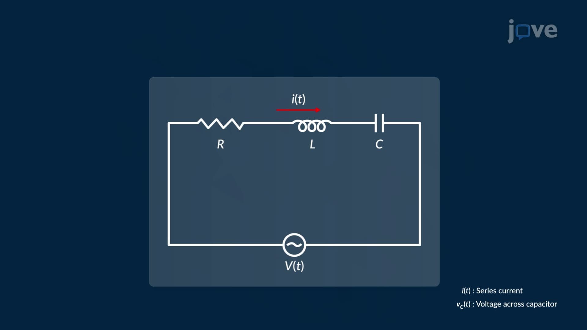
Integration Techniques form the backbone of Calculus 2, equipping students with powerful tools to evaluate complex integrals that basic formulas cannot handle. This micro-course, supported by JoVE Coach, covers advanced integration techniques including integration by parts, trigonometric substitution, partial fractions, improper integrals, and numerical methods — all grounded in real US engineering, physics, and signal-processing applications.

• Understand the integration by parts formula and how it extends from the product rule of differentiation
• Apply integration by parts to both indefinite and definite integrals, including the efficient tabular method for repeated iterations
• Identify the correct strategy for integrating products of powers of sine, cosine, secant, and tangent based on whether exponents are odd or even
• Learn how trigonometric substitution eliminates square root expressions by converting them into manageable trigonometric forms
• Analyze rational functions to determine whether partial fraction decomposition or polynomial long division is the appropriate first step
• Explore rationalizing substitutions that transform non-rational integrands into solvable polynomial expressions
• Apply numerical approximation methods — including the Trapezoidal Rule and Simpson's Rule — when exact antiderivatives are unavailable or data is discrete
• Understand how to evaluate improper integrals over infinite intervals or at points of discontinuity using limit-based definitions

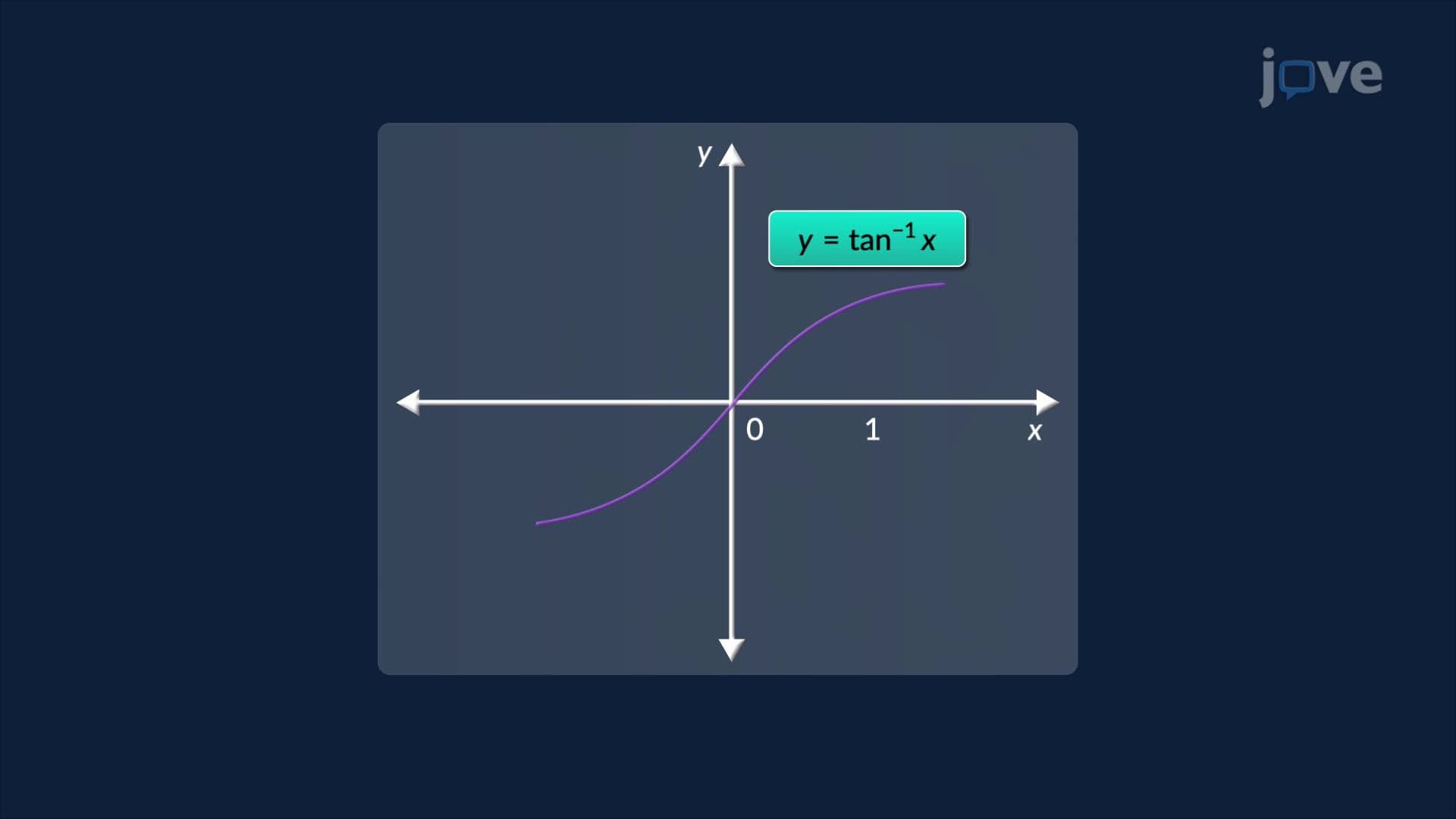
1. Integration by Parts: Indefinite and Definite Integrals Integration by parts is derived from the product rule and follows the formula ∫u dv = uv − ∫v du. Choosing u as the function that simplifies when differentiated — and dv as the remainder — is the critical first step. For definite integrals, the uv term is evaluated at the interval's endpoints before solving the remaining integral. A classic example is integrating the inverse tangent function, which has no standard antiderivative and must be treated as a product with the constant 1. This technique appears in AC circuit analysis, where voltage across a capacitor is found by integrating a product of current-related functions.

2. Integration by Parts: Tabular Method and Problem Solving When integration by parts must be applied multiple times, the tabular method organizes the process efficiently. The integrand is split into an algebraic function (repeatedly differentiated until it reaches zero) and a trigonometric function (repeatedly integrated). Diagonal products are summed with alternating signs to build the antiderivative in one structured pass. This method is especially valuable in signal processing — smart speakers, for example, analyze voice commands by integrating piecewise audio signals multiplied by cosine functions. The tabular approach prevents computational errors and significantly reduces the steps needed for higher-degree polynomial-trigonometric products.

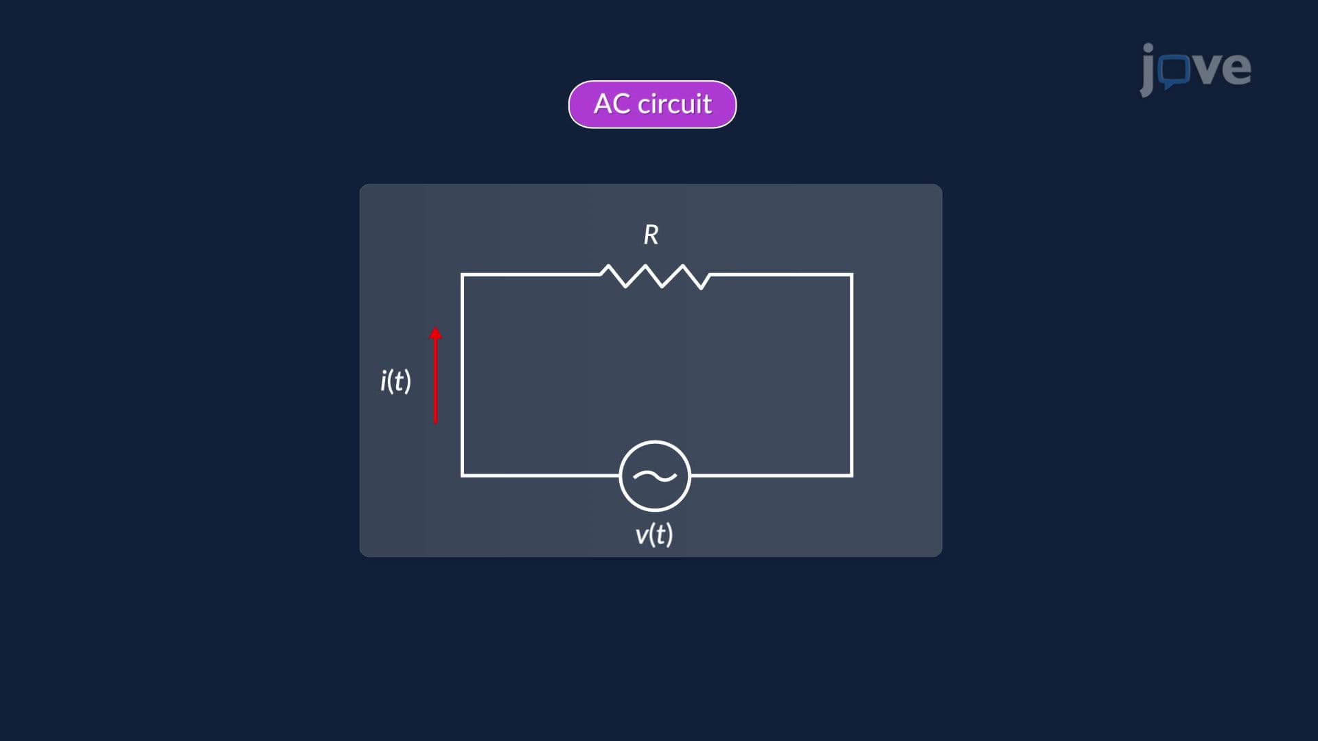
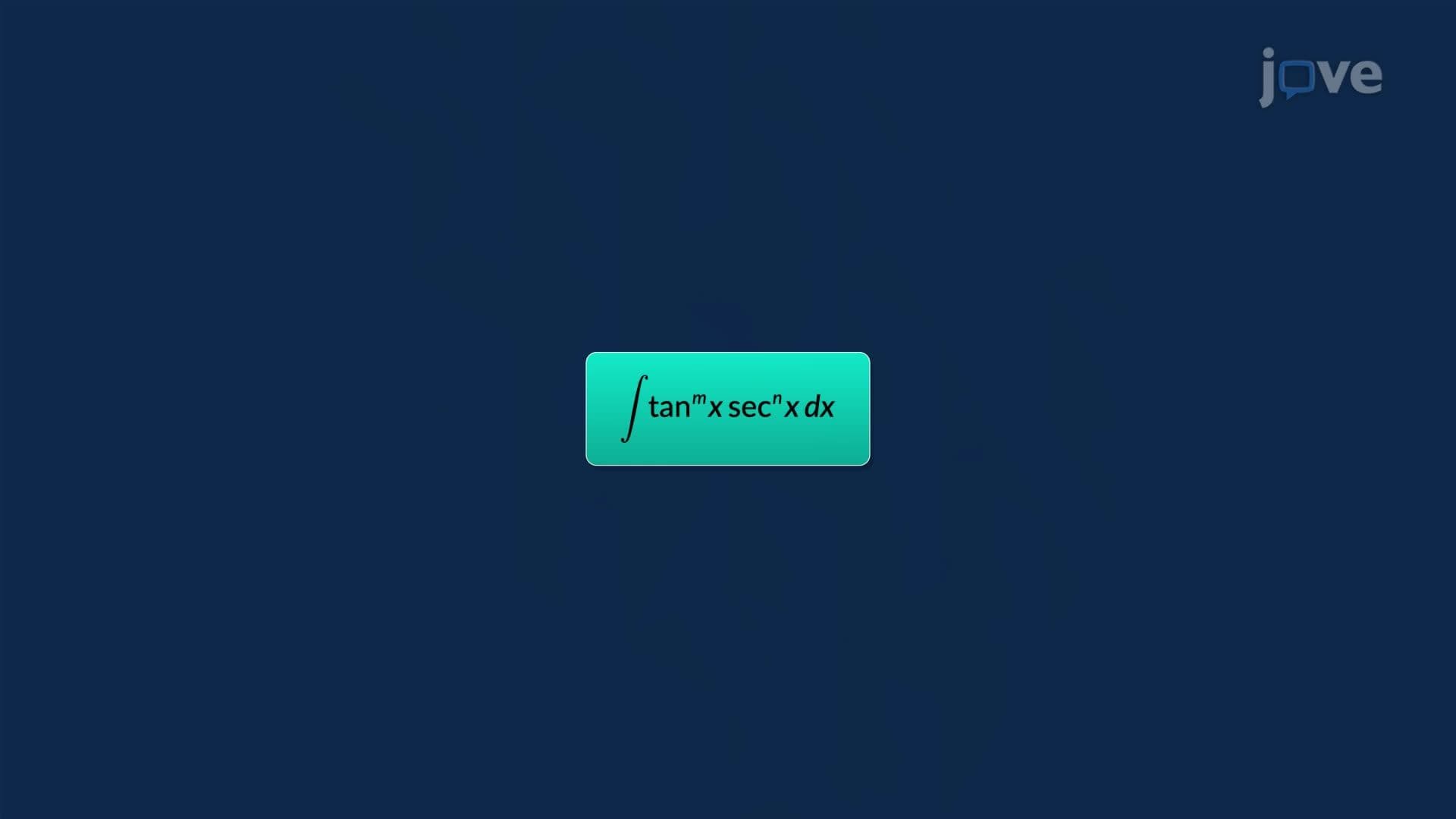
3. Trigonometric Integrals: Powers of Sine, Cosine, Secant, and Tangent For integrals involving sinᵐx cosⁿx, the strategy depends on parity. When one exponent is odd, factor out one copy of that function, convert the remaining even power using a Pythagorean identity, then substitute. When both exponents are even, apply half-angle identities to reduce the powers. Similarly, integrals of secant and tangent functions use substitution guided by whether the secant's power is even or the tangent's power is odd, with Pythagorean identities converting between the two functions. These techniques are used in AC power analysis, where average power in a resistive circuit requires integrating even powers of sinusoidal voltage and current.

4. Trigonometric Substitution Trigonometric substitution replaces algebraic expressions involving square roots — such as √(a² − x²), √(a² + x²), or √(x² − a²) — with trigonometric identities that eliminate the radical. For example, substituting x = a sinθ converts √(a² − x²) into a cosθ, turning a difficult square-root integral into a straightforward trigonometric one. Integration limits are updated to match the new angular variable. A practical US application is computing the total area enclosed by an elliptical satellite orbit, such as those used by Molniya-type communication satellites, where the area formula involves integrating a square-root expression over a symmetric region.

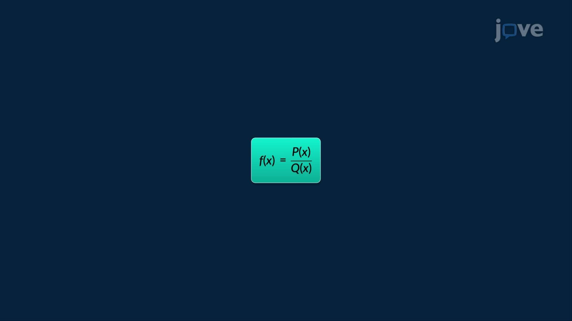
5. Partial Fractions and Integration of Rational Functions Rational functions — ratios of polynomials — are integrated by first classifying them as proper (numerator degree less than denominator) or improper (numerator degree greater than or equal to denominator). Improper rational functions require polynomial long division before decomposition. Proper fractions are decomposed into partial fractions: the denominator is factored, unknown coefficients are introduced for each factor, and substituting strategic values of x solves for those coefficients. Each resulting term integrates cleanly into logarithmic or algebraic expressions. This method is widely used in control systems and electrical engineering, where transfer functions are rational expressions that must be integrated or inverse-transformed.

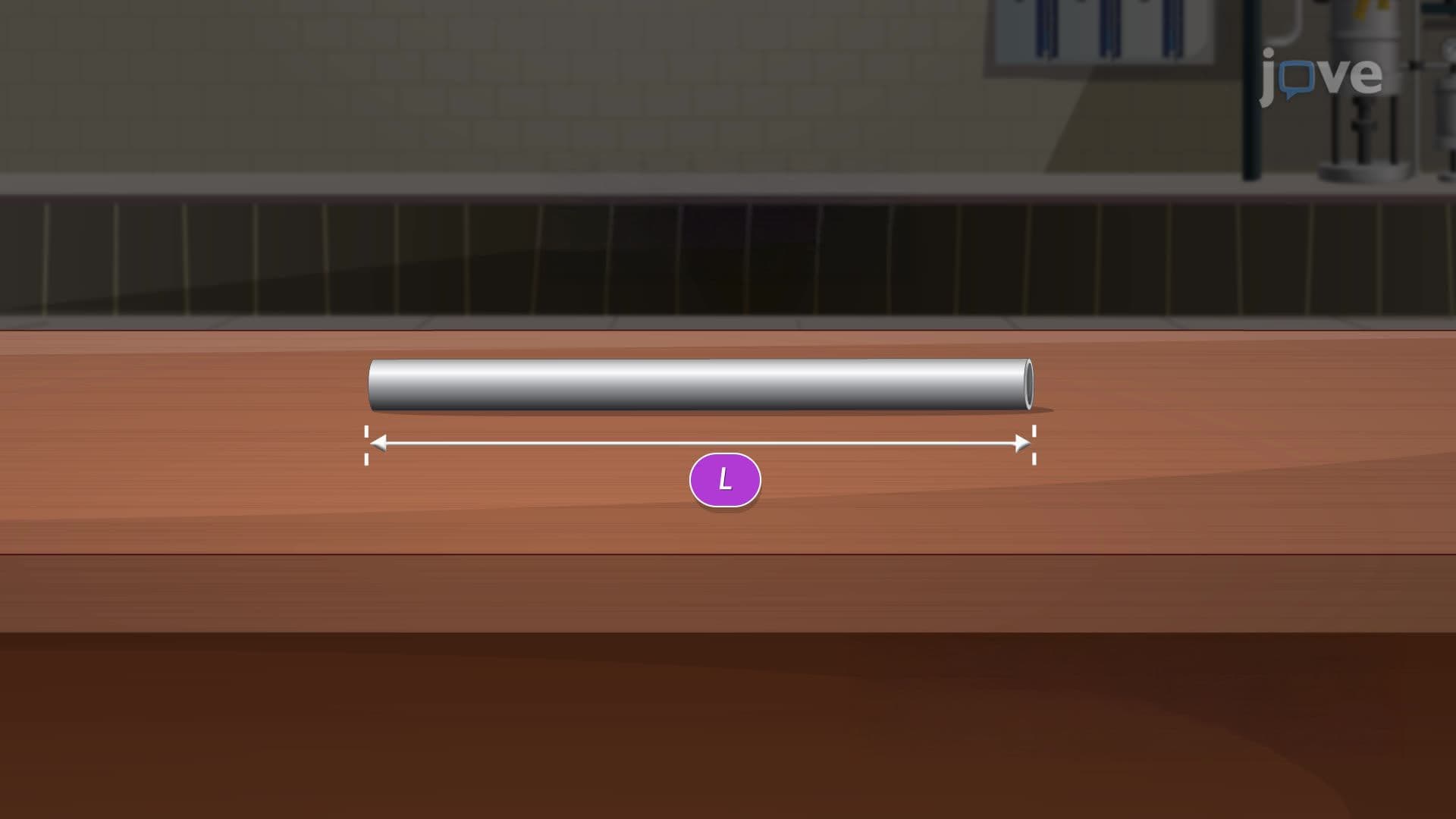
6. Rationalizing Substitutions When an integrand contains irrational expressions such as cube roots or other non-integer radicals, a rationalizing substitution converts the integral into a rational function that can be solved with standard methods. Setting u equal to the root expression eliminates the radical, and dx is rewritten in terms of du. Integration limits are updated accordingly. The resulting rational function may then require polynomial long division before integration. A concrete example is finding the mass of a rod with a density function involving cube roots of distance, a scenario common in materials science and structural engineering problems encountered in undergraduate physics courses.

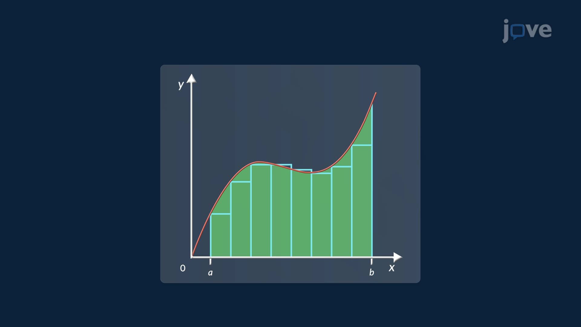
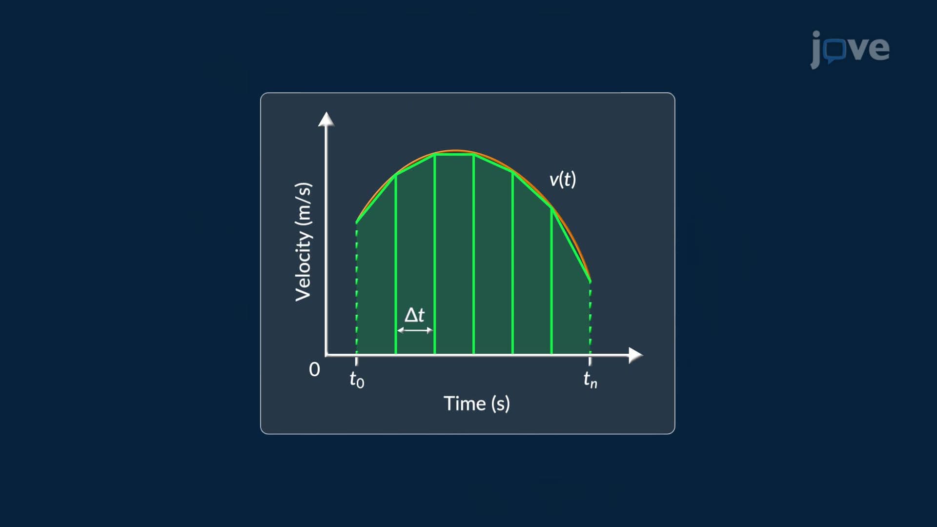
7. Approximate Integration: Riemann Sums, Trapezoidal Rule, and Simpson's Rule When an exact antiderivative cannot be found — or when data comes from discrete measurements rather than a formula — numerical methods estimate definite integrals. Riemann sums use rectangles, with left or right endpoint heights providing lower or upper bounds. The Trapezoidal Rule connects consecutive data points with straight lines, forming trapezoids whose areas sum to an approximation; interior values are counted twice. Simpson's Rule fits parabolas through consecutive triplets of equally spaced points, producing higher accuracy with the same number of sample points. Applications include estimating a truck's displacement from recorded speed data or calculating the surface area of curved warehouse roofing for material cost estimation.

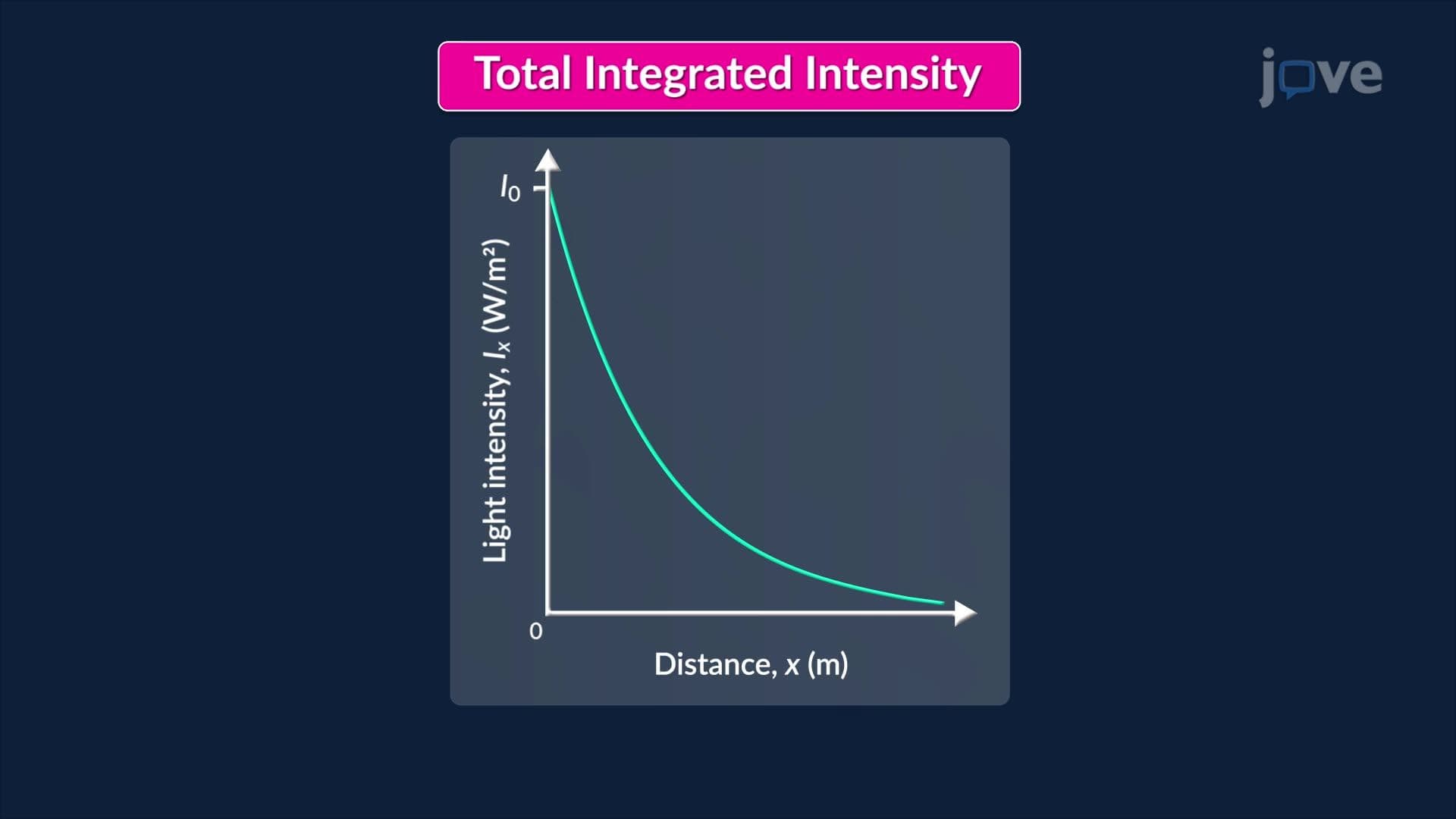
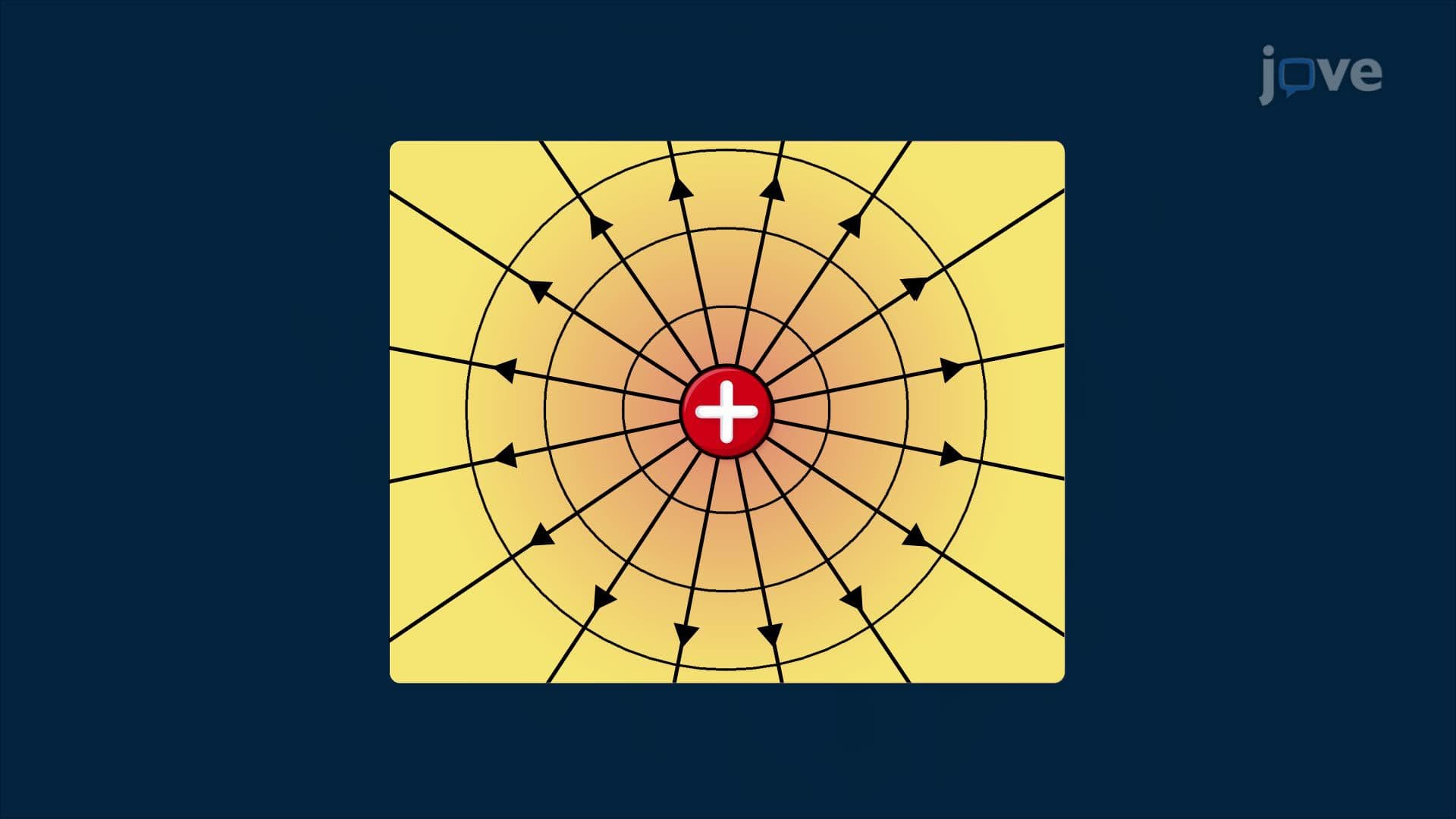
8. Improper Integrals: Infinite Intervals and Discontinuous Integrands An integral is improper either when one or both limits extend to infinity or when the integrand has a vertical asymptote within or at the boundary of the integration interval. Both cases are handled by replacing the problematic bound with a variable and evaluating the result as a limit. If the limit exists and is finite, the integral converges; otherwise, it diverges. Infinite-interval improper integrals model phenomena like the total intensity of light passing through fog over an unbounded distance. Discontinuous-integrand improper integrals appear in electrostatics — for example, computing the electric potential difference of a radial field that becomes infinite near a charged point source.