Loading video…

 14 Concepts
 4.7K views

Video Summary: What Is Approximate Integration
Ever wondered how NASA engineers estimate fuel consumption when sensor data comes in as scattered points rather than a clean formula? That's exactly where approximate integration becomes essential. Approximate integration basics explain how definite integrals are estimated using Riemann sums, dividing intervals into rectangles, when standard antiderivatives fail or data is purely experimental. Watch the full video on JoVE Coach to master this concept with expert-led visuals and step-by-step explanations.
In a perfect mathematical world, every function has a clean antiderivative you can compute symbolically. In reality, that's rarely the case. Approximate integration is the set of techniques used to estimate the value of a definite integral when an exact analytical solution is unavailable or impractical. This situation arises constantly, in AP Calculus AB and BC exams, in college engineering courses, and in real scientific research where data arrives as a table of numbers rather than a tidy formula.
Understanding approximate integration isn't just about passing a test. It's about developing the mathematical judgment to know when exact methods fail and what to do next.
There are two primary situations where approximate integration becomes necessary.
The first is when the antiderivative doesn't exist in closed form. Functions like e^(x²), sin(x)/x, or √(1 + x³) cannot be integrated using standard techniques such as integration by parts, trigonometric substitution, or partial fractions. These methods, powerful as they are, have hard limits.
The second situation occurs when the function is defined by empirical data rather than a formula. In a US university biology lab, for example, a student might measure oxygen consumption in a test subject at five discrete time points. There's no formula to integrate, only data points. Approximate integration makes it possible to estimate the total quantity (like total oxygen consumed) from that limited information.
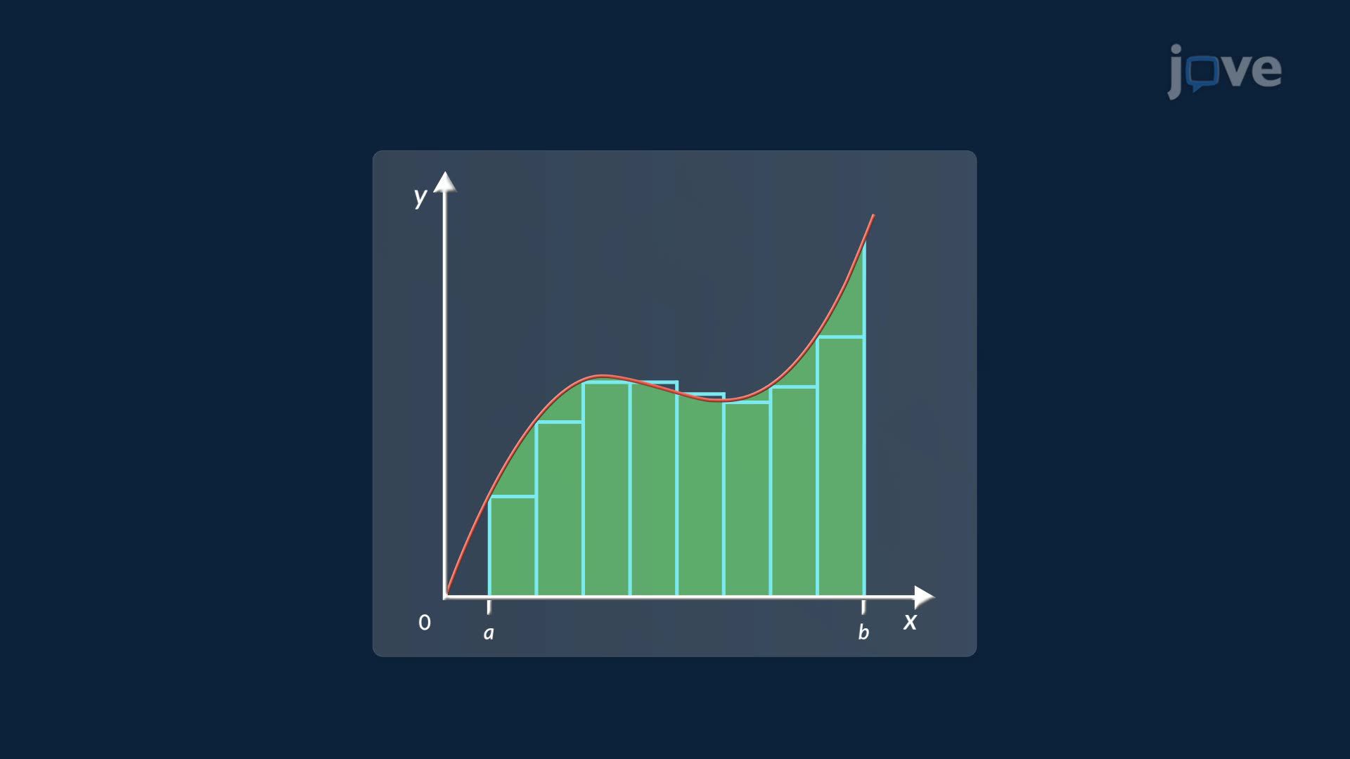
The foundational tool of approximate integration is the Riemann sum. The core idea is elegant: divide the interval [a, b] into n equal subintervals, each with width Δx = (b − a) on n. Over each subinterval, construct a rectangle whose height is determined by the function's value at a chosen point. Add all the rectangle areas together, and you have your estimate of the definite integral.
The left-endpoint approximation (Lₙ) sets each rectangle's height using the function's value at the left end of the subinterval. If the function is increasing over the interval, Lₙ systematically underestimates the true area, because the left-side value is always lower than the actual curve. If the function is decreasing, Lₙ overestimates.
The right-endpoint approximation (Rₙ) does the opposite, it uses the right end of each subinterval. For an increasing function, Rₙ overestimates; for a decreasing function, it underestimates. Recognizing this behavior is a classic question type on AP Calculus exams and college midterms.
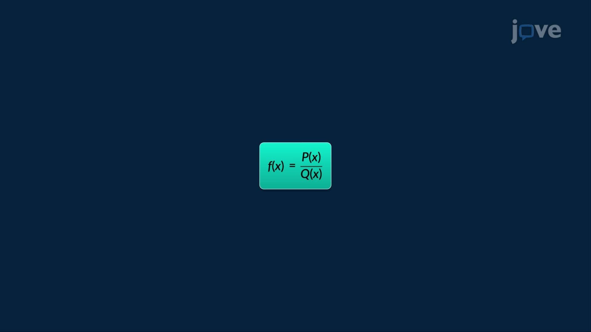
Approximate integration doesn't exist in isolation. It sits within a larger landscape of integration strategies. Before reaching for numerical methods, students typically attempt integration by parts for products of functions, trigonometric substitution for expressions involving square roots, or partial fractions for rational functions. When all analytical roads are blocked, or when dealing with messy real-world data, approximate integration takes over.
On the AP Calculus BC exam, students are regularly expected to use a table of values to compute a Riemann sum estimate. College courses in numerical analysis build directly on these ideas, introducing more precise methods like the Midpoint Rule, Trapezoid Rule, and Simpson's Rule. Mastering the basics of Lₙ and Rₙ now creates a strong foundation for those more advanced tools, and helps students confidently tackle both improper integrals and data-heavy application problems.
Related Micro-courses