Loading video…

 14 Concepts
 4.7K views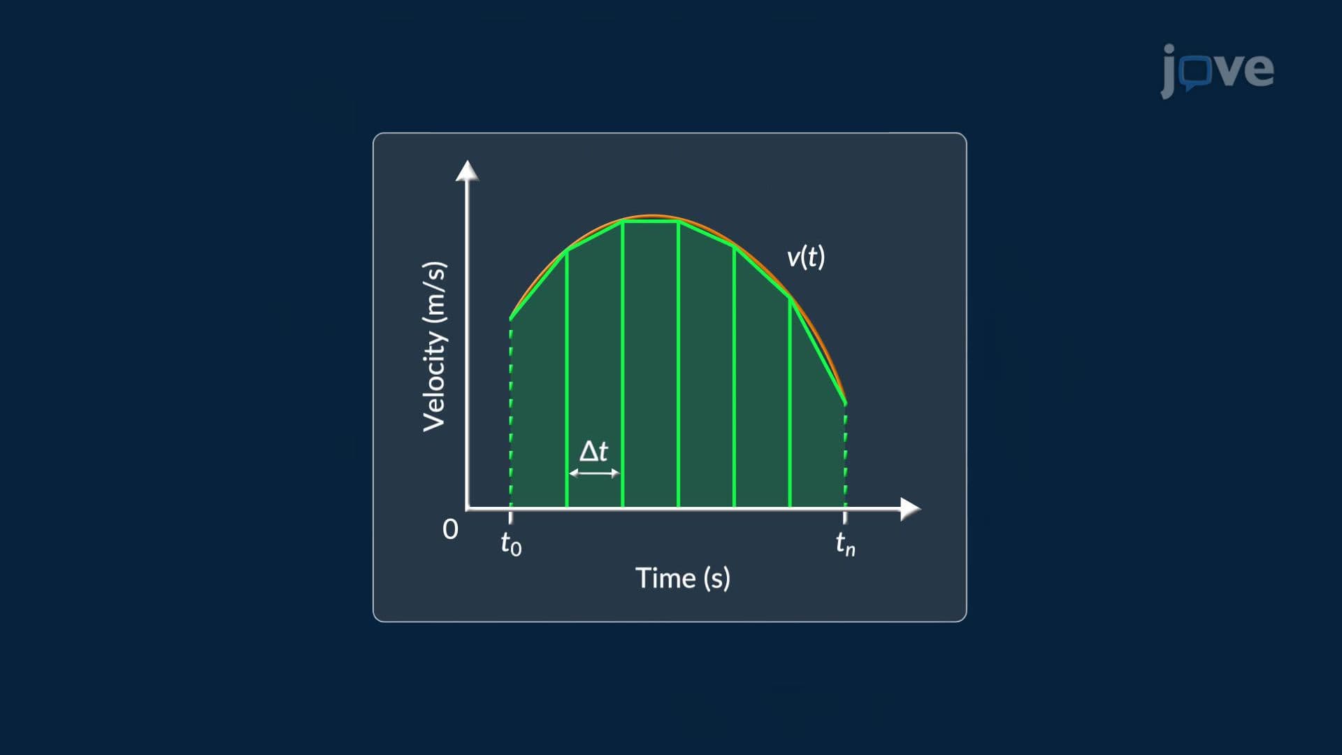

Video Summary: What Is Trapezoidal Rule
How do engineers at NASA estimate fuel consumption when velocity data is only available at specific time intervals? The trapezoidal rule is the answer. What is Trapezoidal Rule? It's a numerical integration method that approximates the area under a curve by dividing it into trapezoids, a technique used in everything from highway traffic analysis to aerospace engineering. Watch the full video on JoVE Coach to master this concept with expert-led visuals and step-by-step explanations.
The trapezoidal rule is a fundamental numerical integration technique used to estimate the definite integral of a function, especially when an exact antiderivative is difficult or impossible to find, or when only discrete data points are available. Rather than computing a precise area under a curve analytically, the trapezoidal rule breaks the interval into smaller segments and approximates each segment as a trapezoid. The areas of all trapezoids are then summed to produce an overall estimate. This approach sits at the intersection of geometry and calculus and forms a critical bridge between theoretical integration and real-world data analysis.
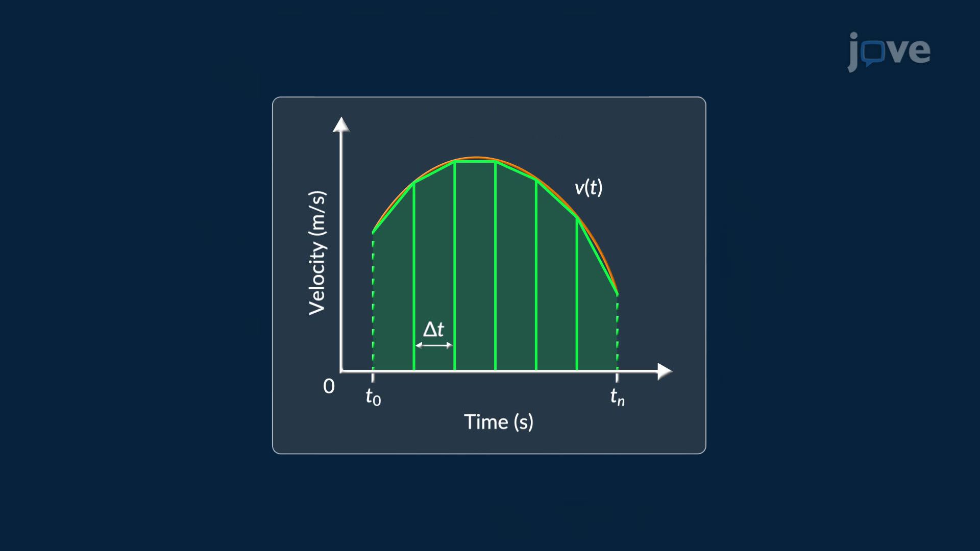
At its core, the trapezoidal rule leverages a simple geometric fact: the area of a trapezoid equals the average of its two parallel sides multiplied by the height (or width, depending on orientation). In the context of a velocity-time graph, the two vertical sides represent velocity values at the start and end of a time subinterval, while the horizontal base represents the time elapsed. By connecting adjacent data points with straight lines instead of curves, the method sacrifices some precision in exchange for computational simplicity, a worthwhile trade in many applied settings.
When the total interval [a, b] is divided into n equal subintervals, each of width Δt = (b − a) / n, the trapezoidal rule formula becomes:
Approximation ≈ (Δt / 2) × [f(t0) + 2f(t1) + 2f(t2) + ... + 2f(t(n−1)) + f(tn)]
Notice that the first value f(t0) and the last value f(tn) appear only once, while every interior value appears twice. This is because each interior point is shared between two adjacent trapezoids, a detail that's frequently tested in AP Calculus exams and college-level numerical methods courses.
The trapezoidal rule isn't just a textbook exercise, it's embedded in professional practice across multiple US industries:
On the AP Calculus AB and BC exams, the trapezoidal rule appears regularly in both multiple-choice and free-response sections. Students are expected to apply it to tables of function values and interpret the result in context. In college calculus courses (Calculus I and II), it often serves as an entry point into broader discussions of numerical integration, error analysis, and comparison with methods like Simpson's Rule.
Understanding the trapezoidal rule also supports comprehension of deeper integration techniques. Students who are comfortable with this method are better prepared to tackle integration by parts, trigonometric substitution, partial fractions, and improper integrals, because each of these methods ultimately seeks the same goal: finding the area under a curve when straightforward formulas fall short. Knowing how to choose an integration technique starts with understanding the nature of the function, and the trapezoidal rule teaches students to think systematically about that choice from the very beginning.
The trapezoidal rule introduces error because straight lines don't perfectly trace curved functions. This error, called truncation error, decreases as n increases (more subintervals = narrower trapezoids = better fit). For concave-up functions, the rule overestimates; for concave-down functions, it underestimates. This relationship to concavity is a concept directly tested in AP Calculus and college midterms, making it essential for students to internalize alongside the formula itself.
Related Micro-courses