Loading video…


 14 Concepts
 4.7K views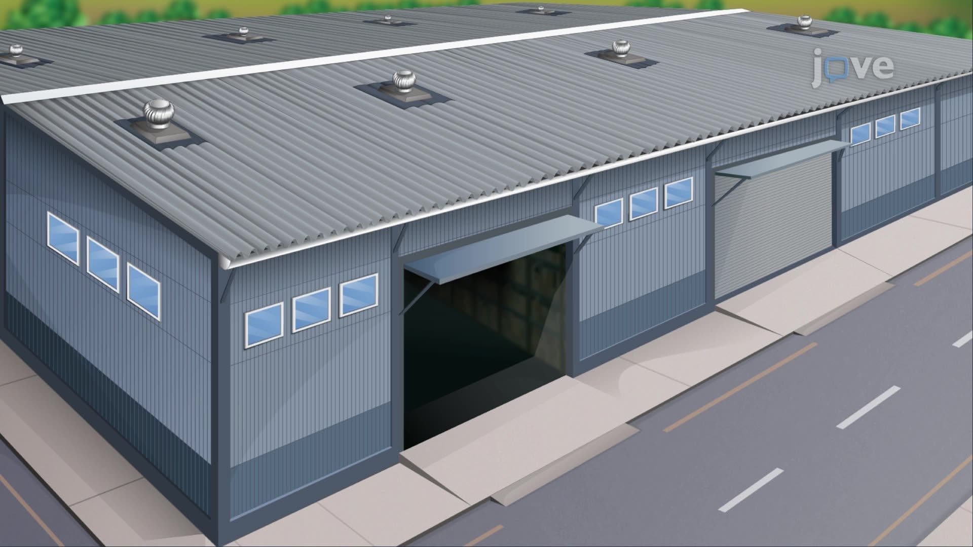

Video Summary: What Is Simpson S Rule Ii
How do engineers know exactly how much metal to order for a curved warehouse roof? Simpson's Rule II provides the answer. This powerful numerical integration method estimates the area under a curve by dividing an interval into even subintervals and applying a repeating coefficient pattern, 1, 4, 2, 4, for remarkable accuracy. US civil engineers regularly use it for material estimation in large-scale construction projects. Watch the full video on JoVE Coach to master this concept with expert-led visuals and step-by-step explanations.
Simpson's Rule II is a numerical integration method that estimates the value of a definite integral by approximating the curve with a series of parabolic segments rather than flat rectangles or straight-line trapezoids. Unlike the Riemann sum or the Trapezoidal Rule, which can introduce significant error with irregular curves, Simpson's Rule II fits a quadratic polynomial through every three consecutive points, capturing the natural curvature of the function and producing a far more accurate result with fewer subintervals.
To apply Simpson's Rule II, you start by identifying two endpoints, call them a and b, that define your total interval on the x-axis. You then divide this interval into n subintervals of equal width, where the width h = (b − a) on n. The critical rule: n must be an even number. This requirement exists because the method pairs subintervals, using every two consecutive subintervals (defined by three equally spaced points) as one parabolic segment. If n were odd, you would be left with an unpaired subinterval, and the method would break down. This is a commonly tested detail on AP Calculus AB and BC exams and college midterms alike.
Once the interval is divided, each function value at the equally spaced points receives a coefficient. The outermost points, f(a) and f(b), receive a coefficient of 1. Every interior point at an even-numbered position receives a coefficient of 2, and every interior point at an odd-numbered position receives a coefficient of 4. This creates the iconic repeating pattern: 1, 4, 2, 4, 2, …, 4, 1. The entire weighted sum is then multiplied by h on 3. This formula is derived by integrating the Lagrange interpolating polynomial that passes through each set of three consecutive points, a process rooted in polynomial algebra and definite integration. Understanding this derivation deepens your grasp of why the method works, not just how to apply it.
Simpson's Rule II appears in surprisingly practical places. Civil and structural engineers at firms across the US, from designing corrugated steel roofing in industrial warehouses in Texas to calculating load distributions on curved highway bridges in California, use numerical integration methods like this when exact analytical solutions are difficult or impossible to compute. In environmental science, it is used to estimate the volume of water in irregularly shaped reservoirs. In AP Physics and college-level engineering courses, students encounter it when analyzing work done by variable forces or computing center-of-mass problems. Wherever a function is complex, noisy, or only known at discrete data points, Simpson's Rule II delivers reliable estimates.
Mastering Simpson's Rule II builds critical intuition for the wider landscape of calculus. It reinforces your understanding of definite integrals, sets the stage for exploring improper integrals, and shows why polynomial approximation is so powerful. It also complements analytical techniques: when you later study integration by parts, trigonometric substitution, trigonometric integrals, or partial fractions for rational functions, you will appreciate that numerical methods like Simpson's Rule II serve as a verification tool, a way to check whether your analytical answer is in the right ballpark. On AP Calculus BC exams and college calculus midterms, problems often ask you to both compute an integral analytically and estimate it numerically, making fluency in both approaches essential.
Related Micro-courses