Parametric Equations and Polar Coordinates

Parametric and polar coordinates form a critical bridge between algebra and advanced calculus. This micro-course, supported by JoVE Coach, covers parametric equations, tangent slopes, surface areas of revolution, and polar coordinate systems. Students explore graphing polar equations, computing arc length in polar coordinates, and calculating areas of polar curves — skills directly tested on AP Calculus BC exams and foundational to STEM coursework across US universities.

• Understand how parametric equations represent motion by expressing x and y as separate functions of a parameter, with real-world examples like projectile trajectories
• Learn how to find the slope of a parametric curve using the chain rule and identify conditions for horizontal and vertical tangents
• Apply parametric integration techniques to calculate surface areas of revolution, including three-dimensional solids like a torus
• Identify how to convert from polar to rectangular coordinates and vice versa using trigonometric relationships and the Pythagorean theorem
• Explore polar curves such as cardioids and rose curves, analyzing how radius varies with angle to produce complex geometric shapes
• Analyze how integration applied to polar coordinates yields exact area values bounded by polar curves
• Apply arc length formulas in polar coordinates to solve real-world navigation and engineering problems involving spiral paths
• Solve multi-step polar coordinate problems involving rose curves, including finding integration limits and applying trigonometric identities

1. Introduction to Parametric Equations Parametric equations redefine curves by expressing both x and y as separate functions of a third variable, typically time t. Rather than writing y = f(x), a parametric approach uses x = f(t) and y = g(t), which allows precise tracking of position at any given moment. This is essential when an object occupies the same spatial position at two different times — such as a baseball that rises and falls through the same height. Each point on the path is the ordered pair (f(t), g(t)), and the parameter t traces the entire trajectory. This framework is widely used in US physics and engineering courses for modeling projectile motion and robotic movement.

2. Calculus with Parametric Curves: Tangents Finding the slope of a parametric curve requires applying the chain rule. The slope of the tangent line at any point equals dy/dt divided by dx/dt, provided dx/dt ≠ 0. A horizontal tangent occurs when dy/dt = 0 and dx/dt ≠ 0, indicating a local maximum or minimum in the vertical direction. A vertical tangent occurs when dx/dt = 0 and dy/dt ≠ 0. This analysis is essential in AP Calculus BC and college-level calculus courses, where students must interpret the geometric behavior of parametric curves, including the direction and speed of a particle's motion along a defined path.

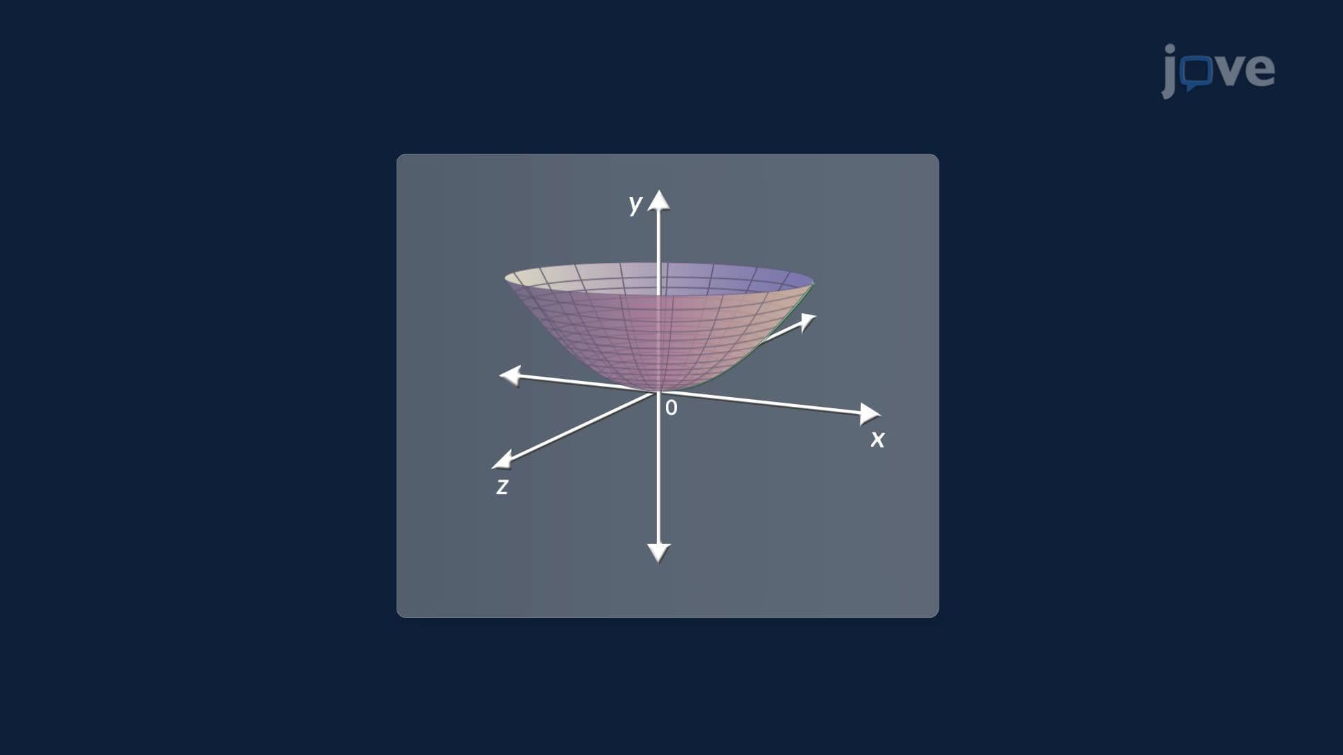
3. Surface Areas of Parametric Curves When a parametric curve is rotated around a coordinate axis, it generates a surface of revolution. The surface area is computed by integrating the product of the circumference of rotation and the arc-length differential over the parameter interval. A classic example is the torus, formed by rotating a circle of radius r centered at distance R from the axis. This technique has direct engineering applications — for instance, calculating the surface area of O-rings used in hydraulic systems and aerospace components. Mastery of this topic prepares students for advanced applied mathematics and is often assessed in college Calculus II courses at US institutions.

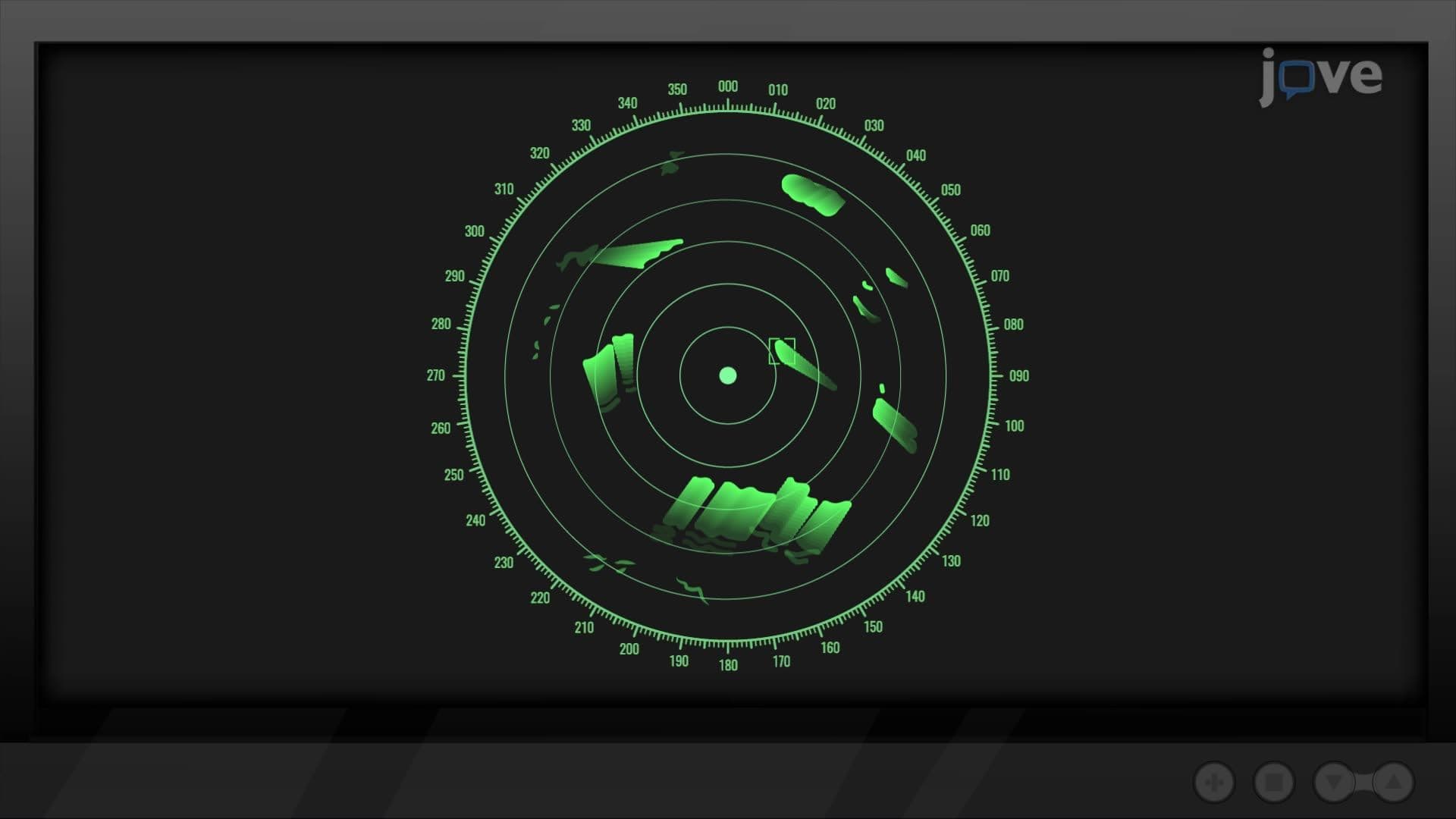
4. The Polar Coordinate System The polar coordinate system locates points using a distance r from a fixed origin (the pole) and an angle θ measured from a reference direction (the polar axis). To convert from polar to rectangular coordinates: x = r cos θ and y = r sin θ. Conversely, r² = x² + y² and tan θ = y/x. A single point can have multiple polar representations — for example, (r, θ) and (−r, θ + π) describe the same location. This system is particularly useful for describing radar systems, circular motion, and antenna broadcast patterns — all common applications in US engineering and physics curricula.

5. Graphing Polar Equations and Polar Curves Polar curves are graphs where the radius r is defined as a function of angle θ. As θ increases from 0 to 2π, the changing values of r trace out distinctive shapes. A cardioid, described by r = 1 + sin θ, forms a smooth, heart-shaped loop. More complex functions generate rose curves with multiple symmetric lobes. Understanding how to interpret and graph these equations is a core skill in AP Calculus BC, where students analyze symmetry, intercepts, and behavior of polar graphs. The spirograph toy — a familiar US classroom manipulative — offers an intuitive entry point into how polar radius and angle interact to produce intricate curves.

6. Area of Polar Curves Using Integration The area enclosed by a polar curve from angle a to b is calculated using A = (1/2)∫[a to b] [r(θ)]² dθ. This formula comes from approximating the region with narrow circular sectors, then taking the limit of Riemann sums. The factor of one-half reflects the proportion of a full circle's area occupied by each sector. This integral technique is applied in fields such as landscape irrigation modeling, radio frequency coverage mapping, and signal analysis — areas where engineers in the US use polar models to quantify non-rectangular regions. AP Calculus BC exams regularly include polar area problems that require identifying correct limits of integration.

7. Arc Length in Polar Coordinates Arc length in polar coordinates is derived by converting polar expressions into rectangular components, differentiating, and then applying the Pythagorean arc-length principle. After squaring and adding the derivatives of x and y with respect to θ, a Pythagorean identity simplifies the expression to: L = ∫√(r² + (dr/dθ)²) dθ. This formula is applied whenever the total distance along a polar curve must be measured — such as calculating the flight path of a drone conducting a spiral search pattern. In US calculus courses, arc length in polar coordinates is a standard Calculus II topic and appears on AP Calculus BC free-response questions.

8. Problem Solving with Polar Coordinates Advanced polar coordinate problems combine multiple skills: identifying zeros of r to find limits of integration, applying trigonometric identities to simplify integrands, and evaluating definite integrals involving squared trigonometric functions. The four-lobed rose curve r = cos(2θ) illustrates this process — each lobe begins and ends at the origin, and integration limits are found by solving r = 0. The half-angle identity for cos²(2θ) then simplifies the integral. These problem-solving strategies are directly applicable to AP Calculus BC exam free-response sections and college placement assessments, where multi-step polar problems test both conceptual understanding and procedural accuracy.