Loading video…


 8 Concepts
 85 views

Video Summary: What are Polar Curves
Ever wonder how a spirograph toy creates those mesmerizing looping patterns? That's the real-world magic behind polar curves. Polar curves basics explain how points are plotted using a radius and an angle instead of x-y coordinates, producing stunning shapes like cardioids and spirals impossible to describe with standard graphing. NASA engineers and roller coaster designers use similar math daily. Watch the full video on JoVE Coach to master this concept with expert-led visuals and step-by-step explanations.
In standard graphing, every point is located by moving horizontally and vertically from an origin, that's the Cartesian system. Polar curves take a completely different approach: every point is described by *how far it is from the center* (the radius, r) and *which direction it faces* (the angle, theta). This shift in perspective unlocks the ability to describe shapes, spirals, loops, petals, and hearts, that would require nightmarishly complex equations in the x-y system but emerge naturally in polar form.
When you graph a polar equation, you're essentially asking: "At each angle, how long is the radius?" Take the classic cardioid equation r = 1 + sin(theta). As theta sweeps from 0 to 2π, the sine function causes r to grow and shrink smoothly, tracing a closed, heart-shaped loop. Change the equation slightly, say, r = 1 + 2sin(theta), and an inner loop appears, producing a limaçon. Swap addition for multiplication and use r = cos(2theta), and you get a four-petaled rose curve. Each small algebraic tweak produces a dramatically different geometric outcome. This direct link between equation structure and curve shape is exactly why graphing polar equations is a core skill in AP Calculus BC and college-level pre-calculus courses across the US.
Because most students first learn Cartesian graphing, knowing how to convert from polar to rectangular coordinates is essential. The conversion formulas are:
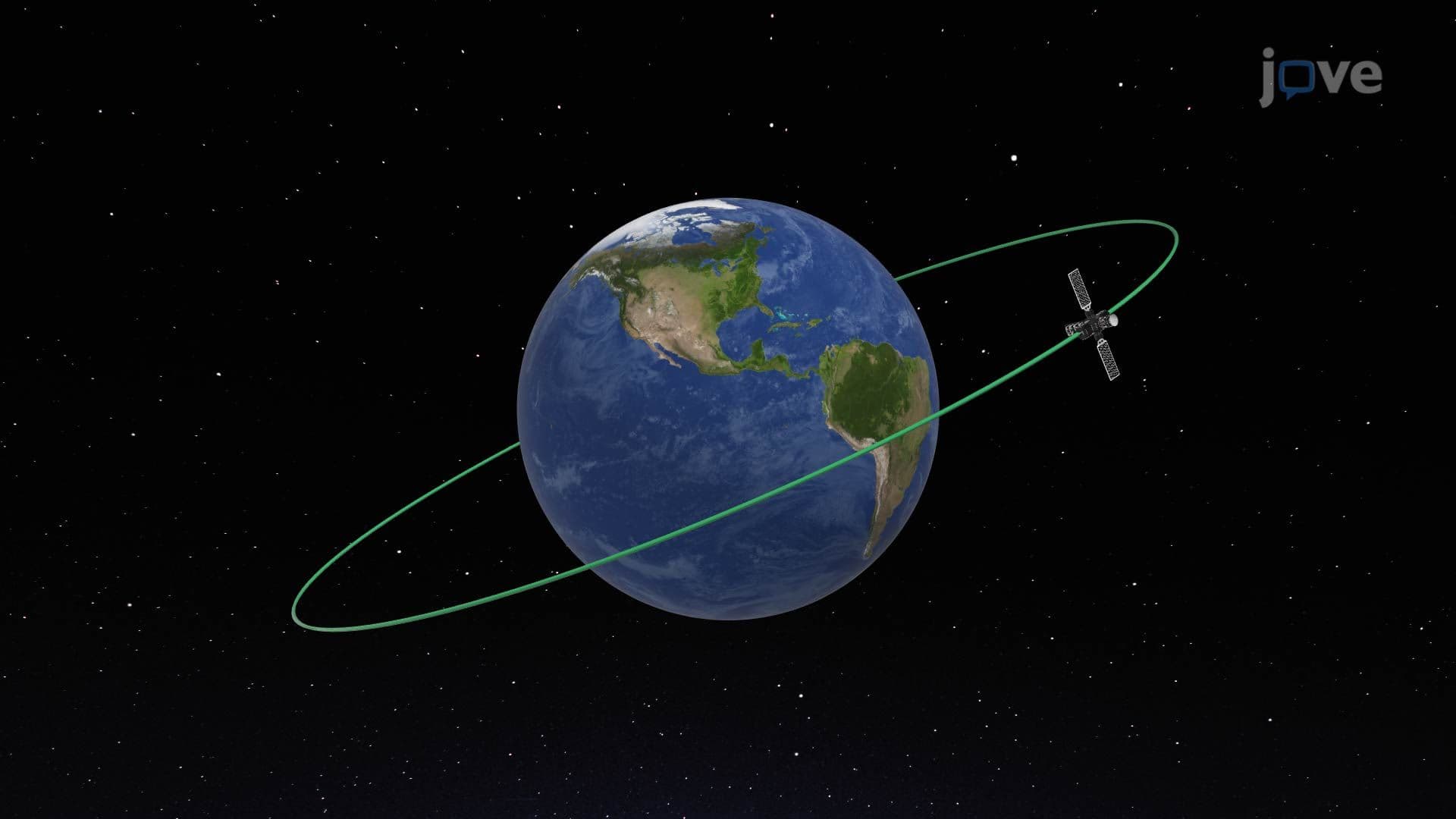
These four relationships act as a bridge between the two systems. For example, the polar equation r = 2 becomes the circle x² + y² = 4 in rectangular form, immediately recognizable. Conversely, conic sections in polar coordinates take elegantly compact forms: an ellipse can be written as r = ed / (1 − e·cos(theta)), where e is eccentricity and d is the directrix distance, a format widely used in orbital mechanics and physics courses at US universities.
Once students reach AP Calculus BC or college Calculus II, polar curves become tools for integration problems. The area of polar curves enclosed by r = f(theta) between angles alpha and beta is:
A = (1/2) · ∫ [r²] dtheta, evaluated from alpha to beta
Similarly, arc length in polar coordinates uses:
L = ∫ sqrt(r² + (dr/dtheta)²) dtheta
Finding the slope of a polar curve, a common AP exam question, requires thinking of it as a parametric curve. Since x = r·cos(theta) and y = r·sin(theta), the slope is dy/dx = (dy/dtheta) / (dx/dtheta), pulling directly from calculus with parametric curves techniques. This interconnection between polar, parametric, and Cartesian representations is a hallmark of advanced high school and introductory college math, and mastering it early creates a significant advantage on AP exams and college midterms.
Related Micro-courses