Loading video…


 8 Concepts
 85 views

Video Summary: Problem Solving in Polar Coordinates
Did you know engineers use math curves to map exactly where a radio tower's signal reaches? Problem solving in polar coordinates makes this possible, and it's more powerful than you might expect. In the US, network planners rely on four-lobed rose curves to model directional broadcast beams, calculating precise coverage areas using polar integration. Watch the full video on JoVE Coach to master this concept with expert-led visuals and step-by-step explanations.
In standard math classes, students work almost exclusively in rectangular coordinates, plotting points as (x, y). But many natural and engineered phenomena, radio signals, planetary orbits, radar sweeps, are fundamentally circular or rotational. That is exactly why problem solving in polar coordinates is such a critical skill. Instead of x and y, polar coordinates use r (the distance from a central point called the pole) and θ (the angle measured from a reference direction). Together, they describe shapes and regions that would require far more complicated equations in rectangular form.
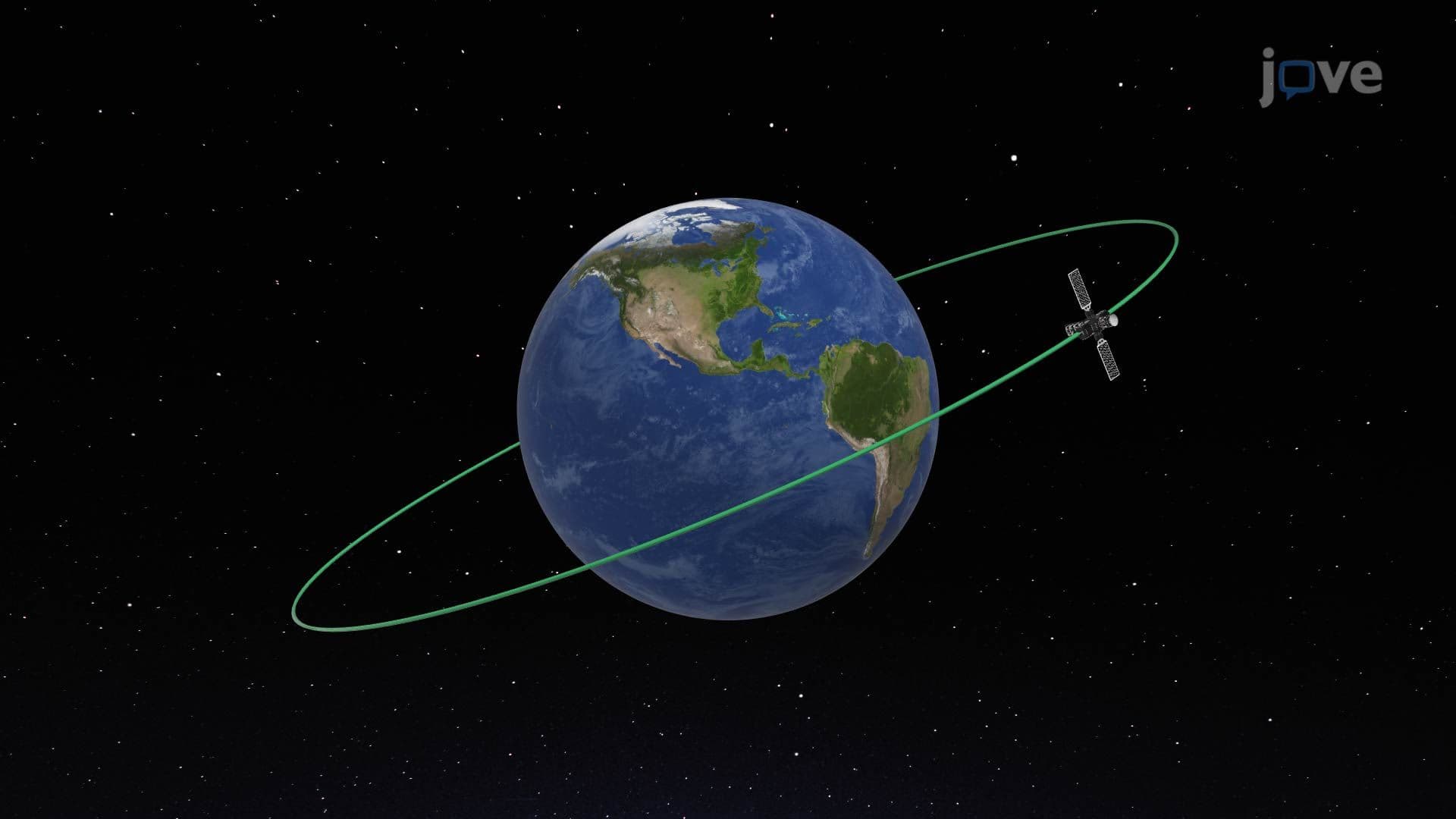
Polar coordinates are widely used across physics, engineering, and applied mathematics. US aerospace engineers at agencies like NASA use polar equations to model orbital paths. Telecommunications companies use them to design antenna patterns and calculate signal coverage areas. In calculus courses across American universities, polar coordinates appear in topics ranging from arc length in polar coordinates to double integrals over circular regions. Even on the AP Calculus BC exam, students are expected to set up and evaluate area integrals in polar form, making this one of the highest-value skills to develop.
One of the most visually striking families of polar curves is the rose curve, expressed as r = a·cos(nθ) or r = a·sin(nθ). When n is even, the rose has 2n petals; when n is odd, it has n petals. The four-lobed rose, r = a·cos(2θ), is a textbook example used in both graphing polar equations exercises and real engineering models for directional antennas. Each petal (or lobe) corresponds to a directional beam, and identifying where r = 0 gives the exact angular boundaries of each lobe, a critical first step before any integration.
The universal formula for the area enclosed by a polar curve between two angles is:
A = (1/2) ∫ r² dθ (integrated from θ = α to θ = β)
This formula comes directly from the idea of summing infinitely thin circular sectors, much like rectangular integration sums infinitely thin rectangles. For a single lobe of r = a·cos(2θ), the lobe exists between θ = -π/4 and θ = π/4, the angles where the curve returns to the origin. Substituting and squaring gives a cos²(2θ) term, which is simplified using the trigonometric reduction identity:
cos²(u) = (1 + cos(2u)) / 2
This identity converts the integral into a form that can be evaluated with standard antiderivative rules, producing the exact area of one signal beam's coverage zone. This same technique, identify limits, substitute, simplify with identities, integrate, applies to virtually every area problem involving polar curves on AP exams and college midterms.
Problem solving in polar coordinates does not exist in isolation. It connects directly to parametric equations examples, since both systems describe curves using indirect relationships rather than direct y = f(x) functions. Students who understand how to find the slope of a parametric curve using dy/dx = (dy/dt)/(dx/dt) can apply similar reasoning to polar tangent lines. Knowing how to convert from polar to rectangular coordinates, using x = r·cos(θ) and y = r·sin(θ), bridges these two powerful systems and deepens conceptual understanding across all of calculus. Mastering these connections now prepares students for multivariable calculus, physics-based math, and standardized exams where these relationships appear repeatedly.
Related Micro-courses