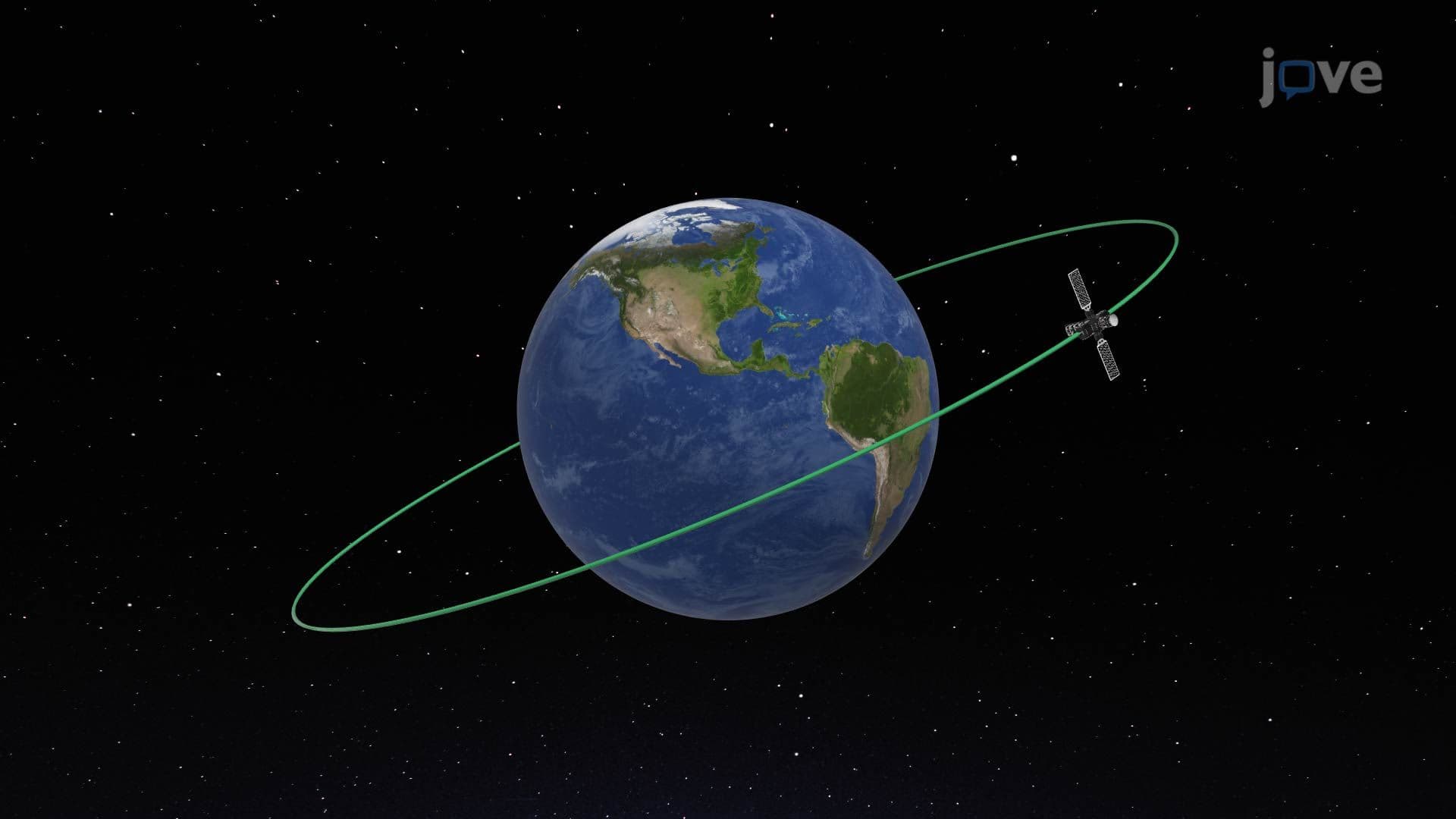
Vector functions and space curves form the mathematical backbone of motion analysis across physics, engineering, and aerospace science. This micro-course, developed with JoVE Coach, covers the calculus of vector-valued functions — from derivatives and integrals to curvature, torsion, and projectile motion. Students explore how NASA engineers, air traffic controllers, and robotics designers use these principles to model real-world three-dimensional motion with precision.

• Understand what vector-valued functions are and how they differ from real-valued functions, including how their component functions define motion in three-dimensional space
• Identify space curves and explain how a moving particle's position traces a path described by a vector function over a given parameter interval
• Apply differentiation and integration techniques to vector functions to find velocity, speed, acceleration, and displacement vectors
• Analyze arc length of a space curve by integrating the magnitude of a position vector's derivative over a specified time interval
• Explore curvature and its geometric interpretation, including how the unit tangent vector and normal vector describe the bending of a curve at any point
• Identify the binormal vector and torsion, and explain how the Frenet–Serret frame describes a curve's full three-dimensional geometry
• Analyze the tangential and normal components of acceleration to understand how speed changes and direction shifts along a curved path
• Apply vector function principles to solve projectile motion and real-world motion problems, including collision prediction and drone navigation scenarios

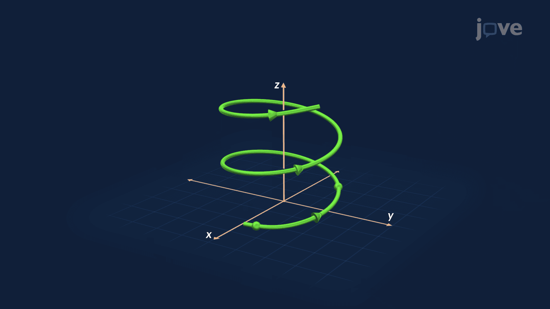
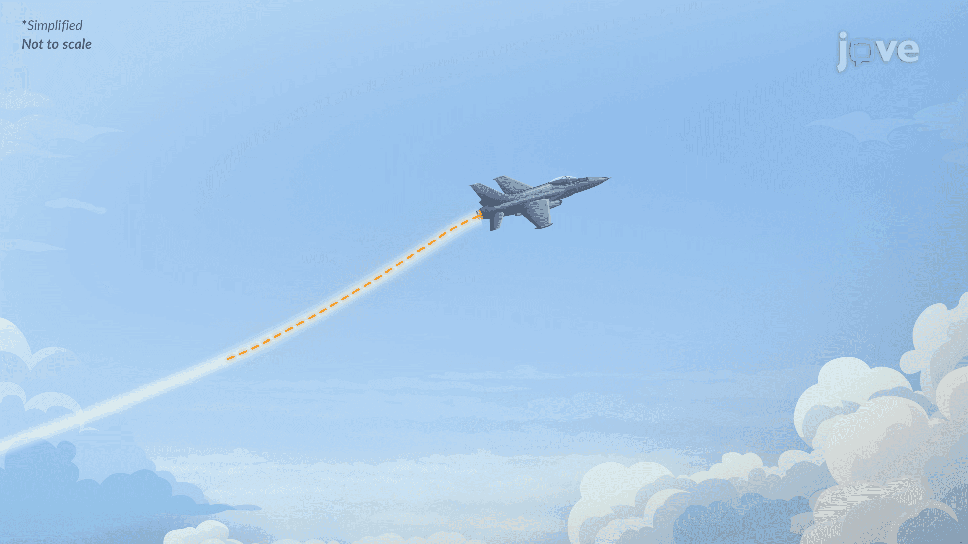
1. Vector-Valued Functions and Space Curves A vector-valued function assigns a unique vector in space to each real-number input, typically time. In three dimensions, three scalar component functions — one for each coordinate axis — work together to describe a particle's position at every moment. As the input changes, the tip of the position vector traces a continuous path called a space curve. A classic example is a three-dimensional helix, where two components trace a circle while the third rises steadily — similar to the flight path of an aircraft climbing through a cloud layer over Chicago O'Hare Airport. Space curves are the geometric objects at the heart of motion analysis.

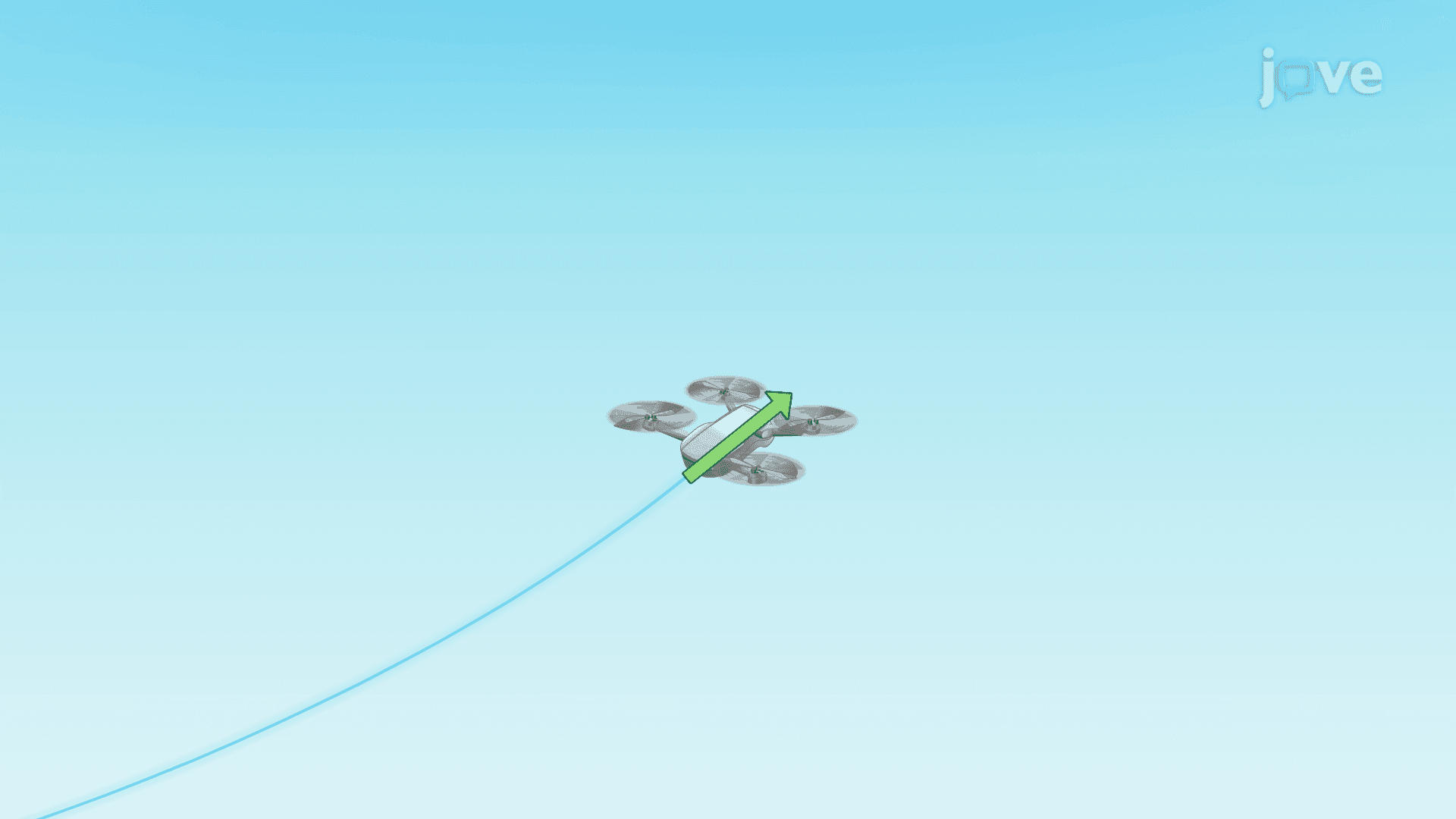
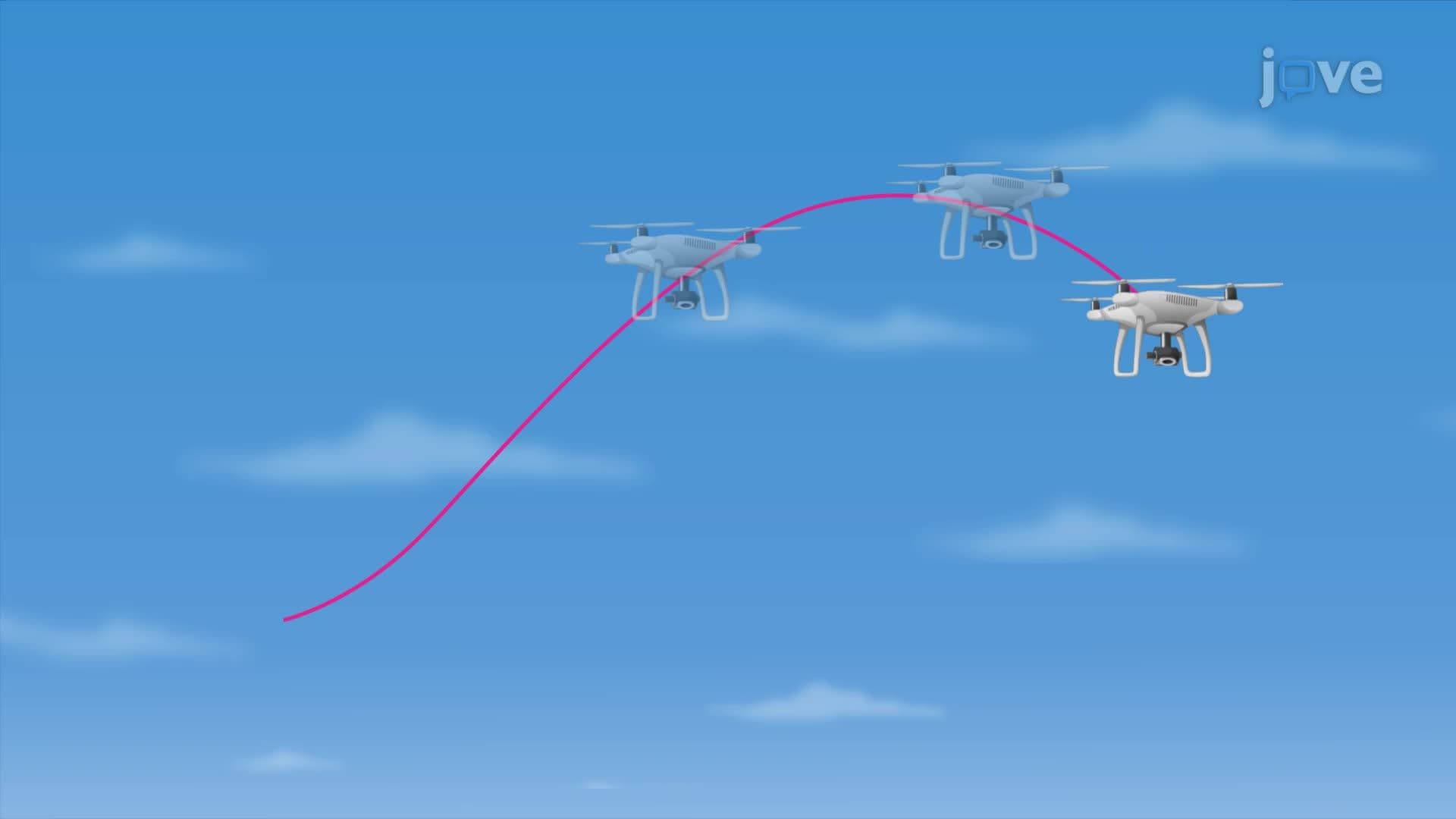
2. Derivatives of Vector Functions: Velocity and Acceleration Differentiating a vector function with respect to time yields the velocity vector, which points tangent to the curve and captures both speed and direction of motion at each instant. Differentiating velocity gives the acceleration vector. Because each component is a real-valued function, differentiation is applied component by component. For example, if a drone's position is described by cubic and quadratic terms in time, the velocity and acceleration vectors are found by standard polynomial differentiation applied to each axis independently. This approach is fundamental in robotics and aerospace engineering for programming autonomous vehicle paths.

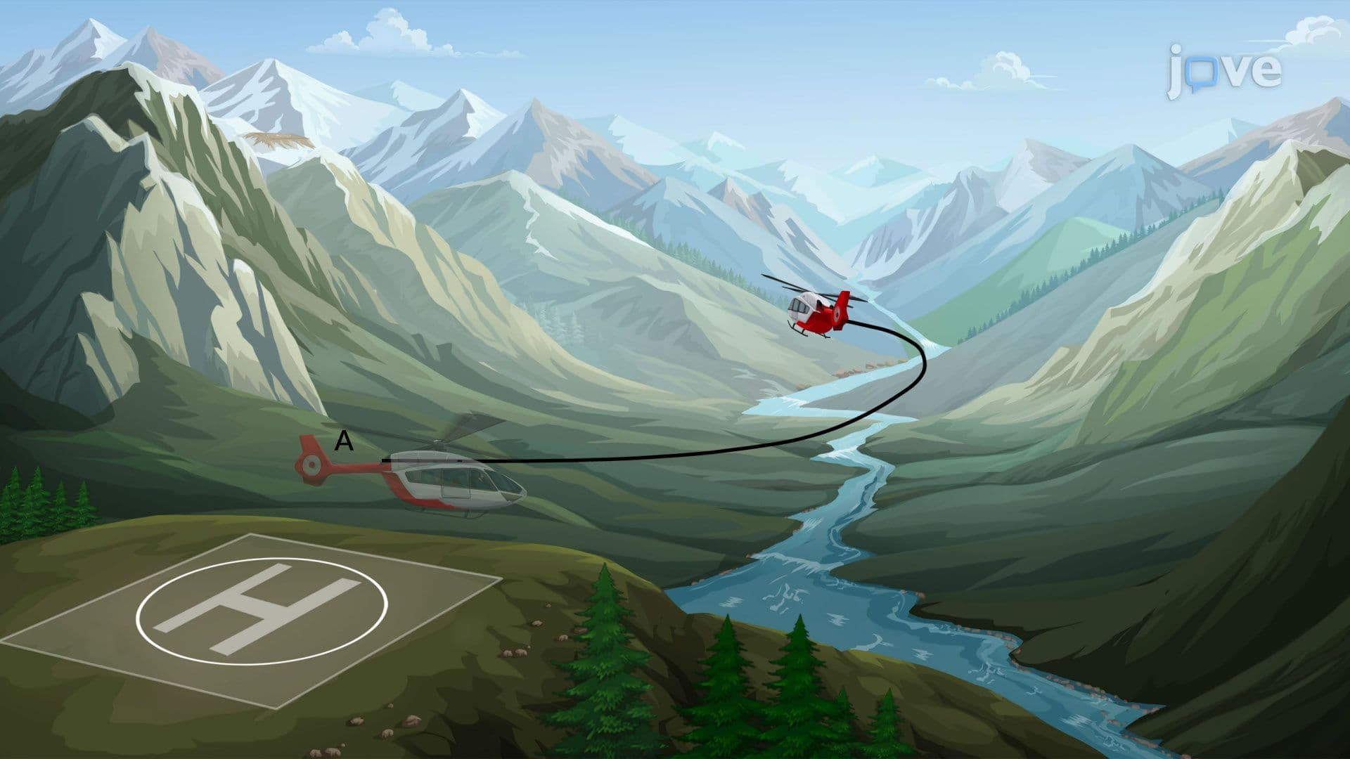
3. Integrals of Vector Functions Integrating a vector-valued function reverses differentiation: integrating a velocity vector recovers the position function, and integrating an acceleration vector recovers velocity. Each component is integrated separately, and initial conditions — the known position or velocity at time zero — are used to determine the constants of integration. In practical terms, if a helicopter's velocity is known as a function of time, integrating component by component gives its displacement vector over any time interval. This technique is used by aerospace engineers when computing a spacecraft's trajectory from thrust data recorded during a launch sequence.

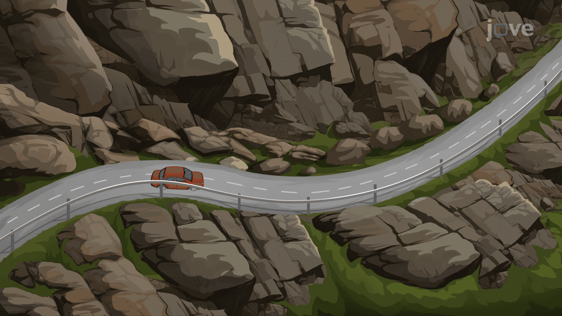
4. Arc Length of a Space Curve The arc length of a space curve measures the actual distance traveled along a curved path — not the straight-line distance between two points. It is computed by integrating the magnitude of the derivative of the position vector over a given time interval. Conceptually, the curve is subdivided into tiny nearly-straight segments; summing their lengths and taking the limit as segment size approaches zero yields the exact arc length formula. This is directly relevant in engineering applications like calculating the cable length needed to run fiber-optic lines along a curved mountain highway in Colorado or determining fuel consumption for a curved helicopter route.

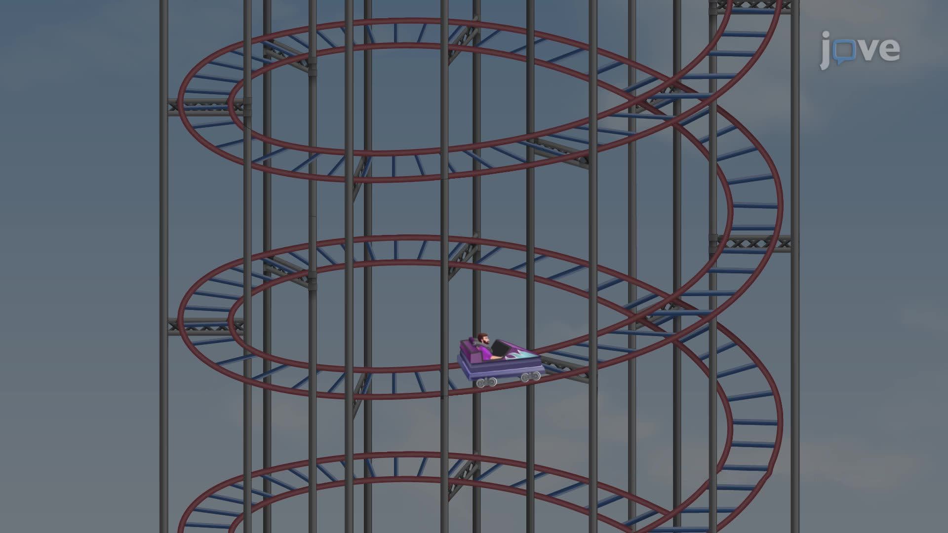
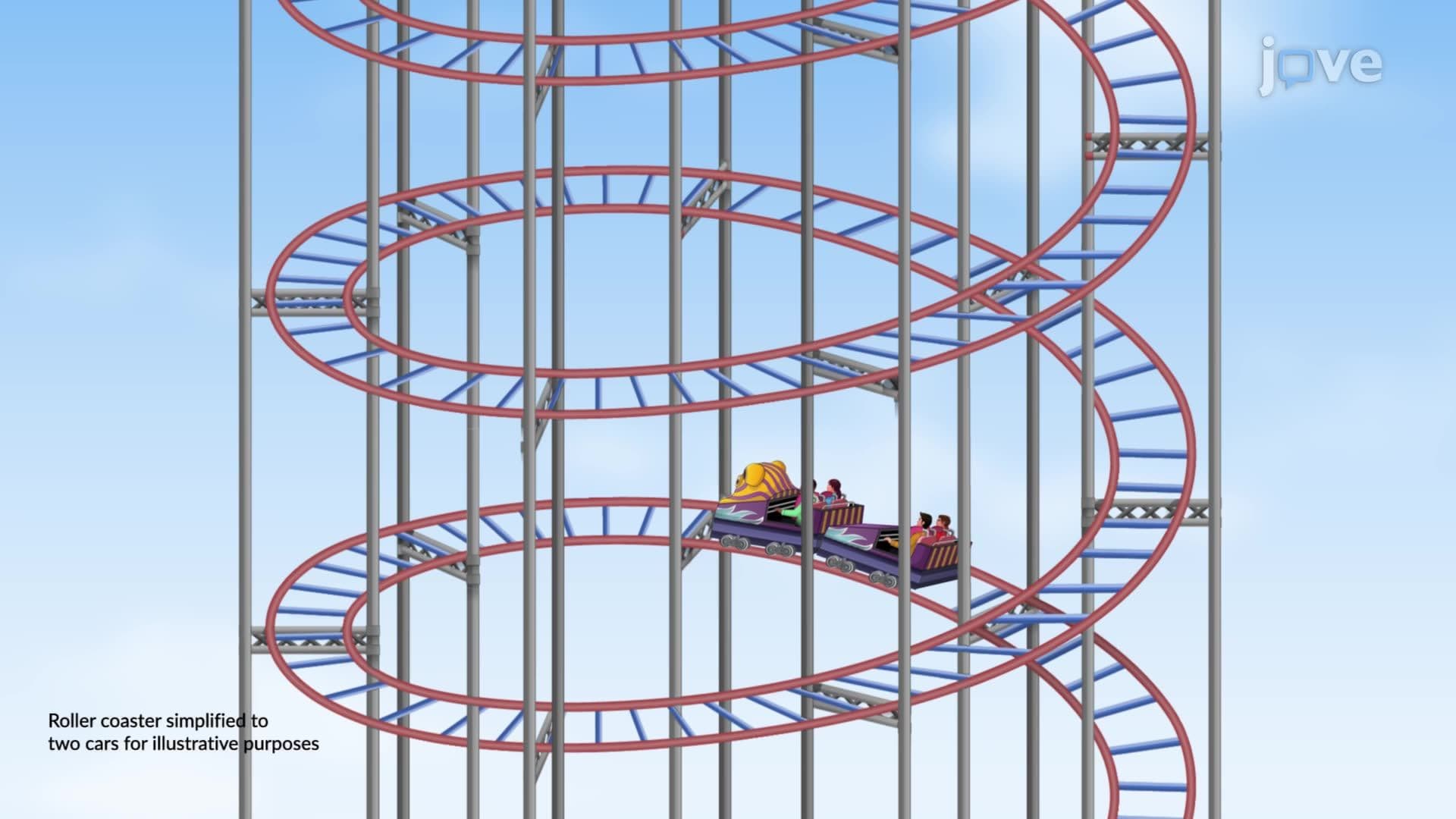
5. Curvature and the Unit Tangent Vector Curvature quantifies how sharply a curve bends at any given point. It is computed as the magnitude of the rate of change of the unit tangent vector with respect to arc length. The unit tangent vector is the normalized first derivative of the position function. A circle with a small radius has high curvature; a nearly straight highway on-ramp has low curvature. For a helix, curvature depends on both the radius and the pitch — increasing the vertical rise per radian decreases curvature. Understanding curvature is essential in road design, roller coaster engineering, and the guidance systems of autonomous vehicles navigating curved terrain.

6. The Normal Vector, Binormal Vector, and the Frenet–Serret Frame Three mutually perpendicular unit vectors — the tangent T, normal N, and binormal B — form a moving coordinate system called the Frenet–Serret frame that travels with a particle along its path. The unit tangent vector points in the direction of motion. The unit normal vector is perpendicular to the tangent and points toward the center of curvature — inward along a turn. The binormal vector, computed as the cross product of T and N, is perpendicular to both and indicates how the curve twists in space. This three-vector system is used in aerospace navigation and in animating realistic camera movements along curved paths in film and game design.

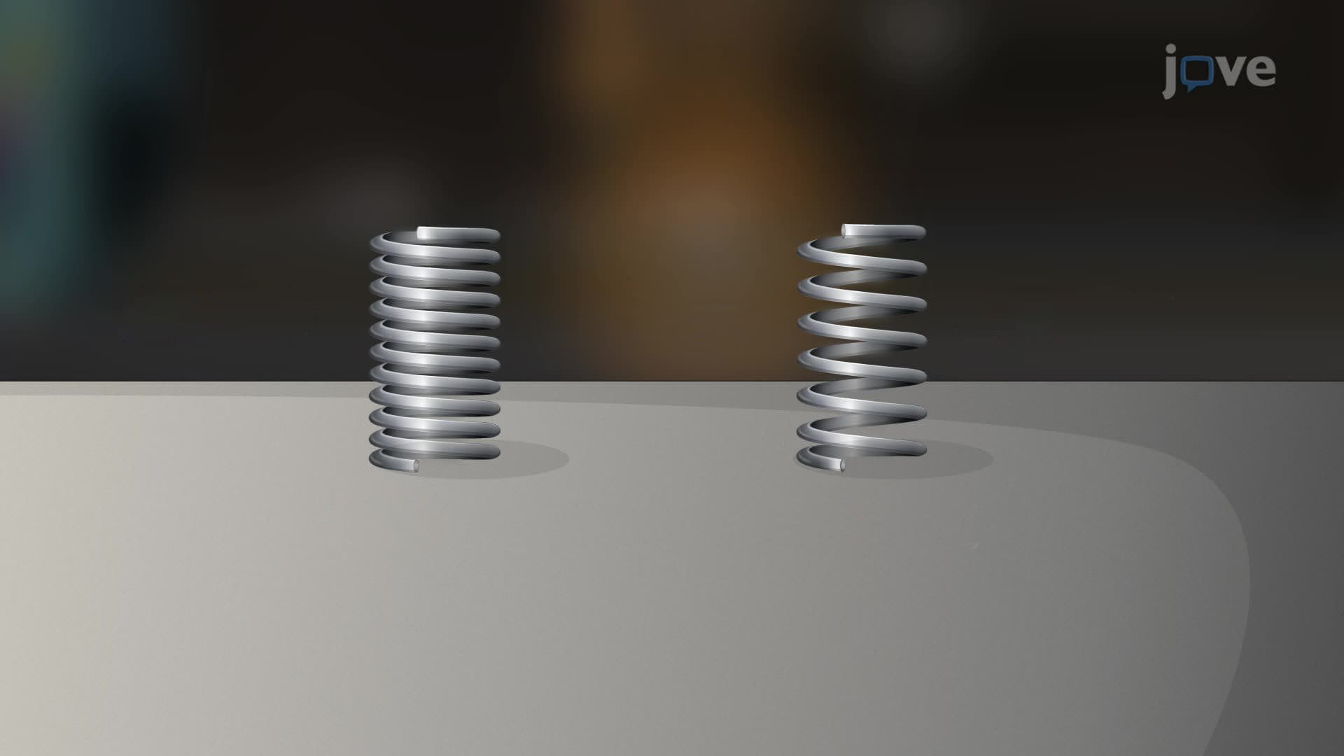
7. Torsion Torsion measures how rapidly a space curve twists out of the plane formed by its tangent and normal vectors — called the osculating plane — per unit of arc length. While curvature captures bending within a plane, torsion captures the three-dimensional twist into the next dimension. When torsion is zero, the curve lies entirely in a single plane with no twisting, like a circular loop. A helix has constant, nonzero torsion, reflecting its steady spiral structure. Torsion appears in structural engineering when analyzing helical springs, in molecular biology when modeling DNA double-helix geometry, and in robotics when planning tool-path orientations for precision machining.

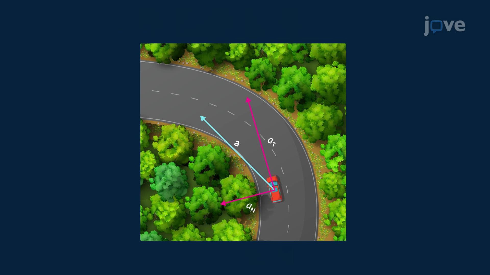
8. Tangential and Normal Components of Acceleration Acceleration along a curved path can be split into two perpendicular parts: the tangential component, which acts along the direction of motion and reflects changes in speed, and the normal component, which acts perpendicular to motion and reflects changes in direction. The normal component depends on both the square of the speed and the curvature of the path. This explains why a sharp turn at high speed produces a strong lateral force — as felt by passengers in a car navigating a tight freeway ramp. Decomposing acceleration this way is critical in vehicle dynamics, roller coaster safety analysis, and the design of banked highway curves by US civil engineers.

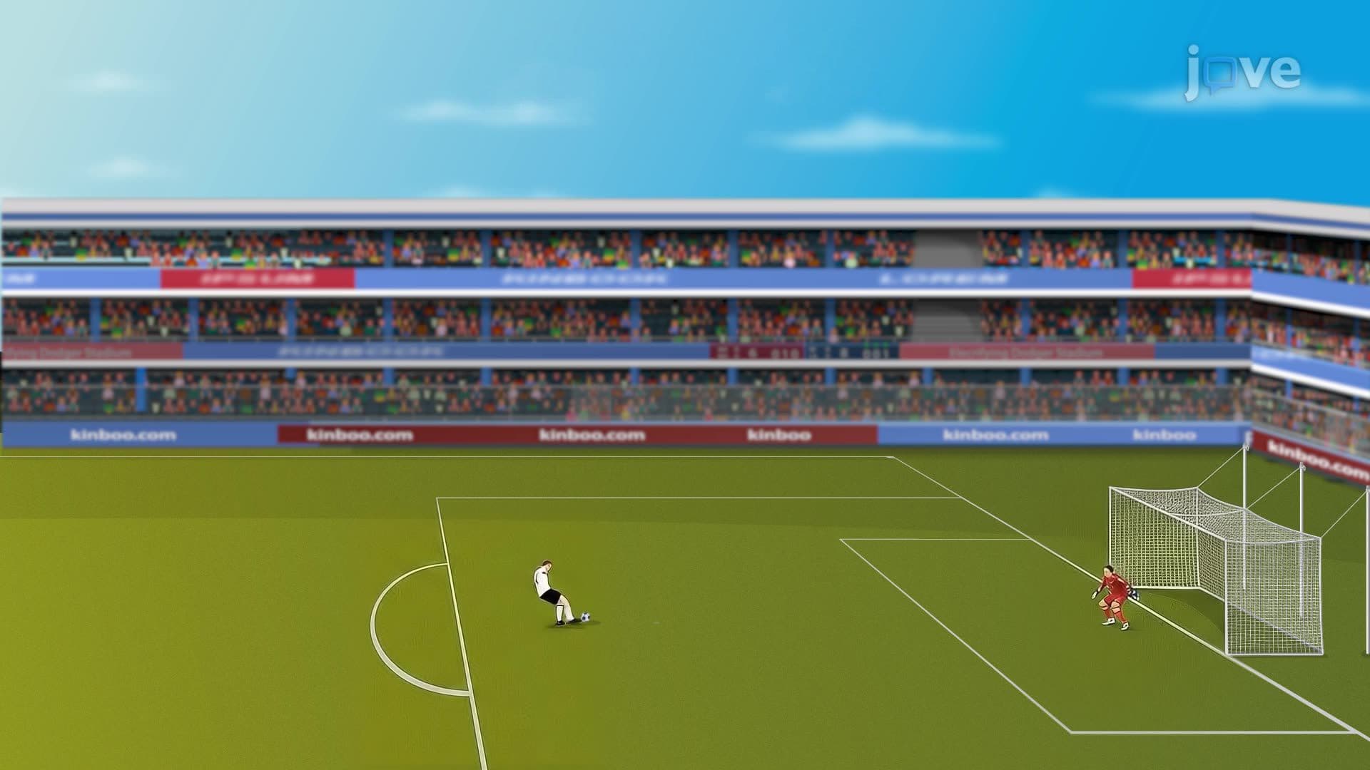
9. Projectile Motion Projectile motion describes the trajectory of an object launched into the air under the influence of gravity alone, with air resistance neglected. The motion is analyzed by decomposing the velocity vector into horizontal and vertical components using the launch angle. Horizontal acceleration is zero, so horizontal velocity stays constant. Vertical acceleration equals the downward gravitational constant. Integrating each component twice gives the position as a function of time. The resulting trajectory is parabolic. This framework is applied in sports science — analyzing a football's flight path during a field goal attempt — and in ballistic engineering for modeling the trajectories of projectiles at facilities like Aberdeen Proving Ground.