Loading video…

 13 Concepts
 47 views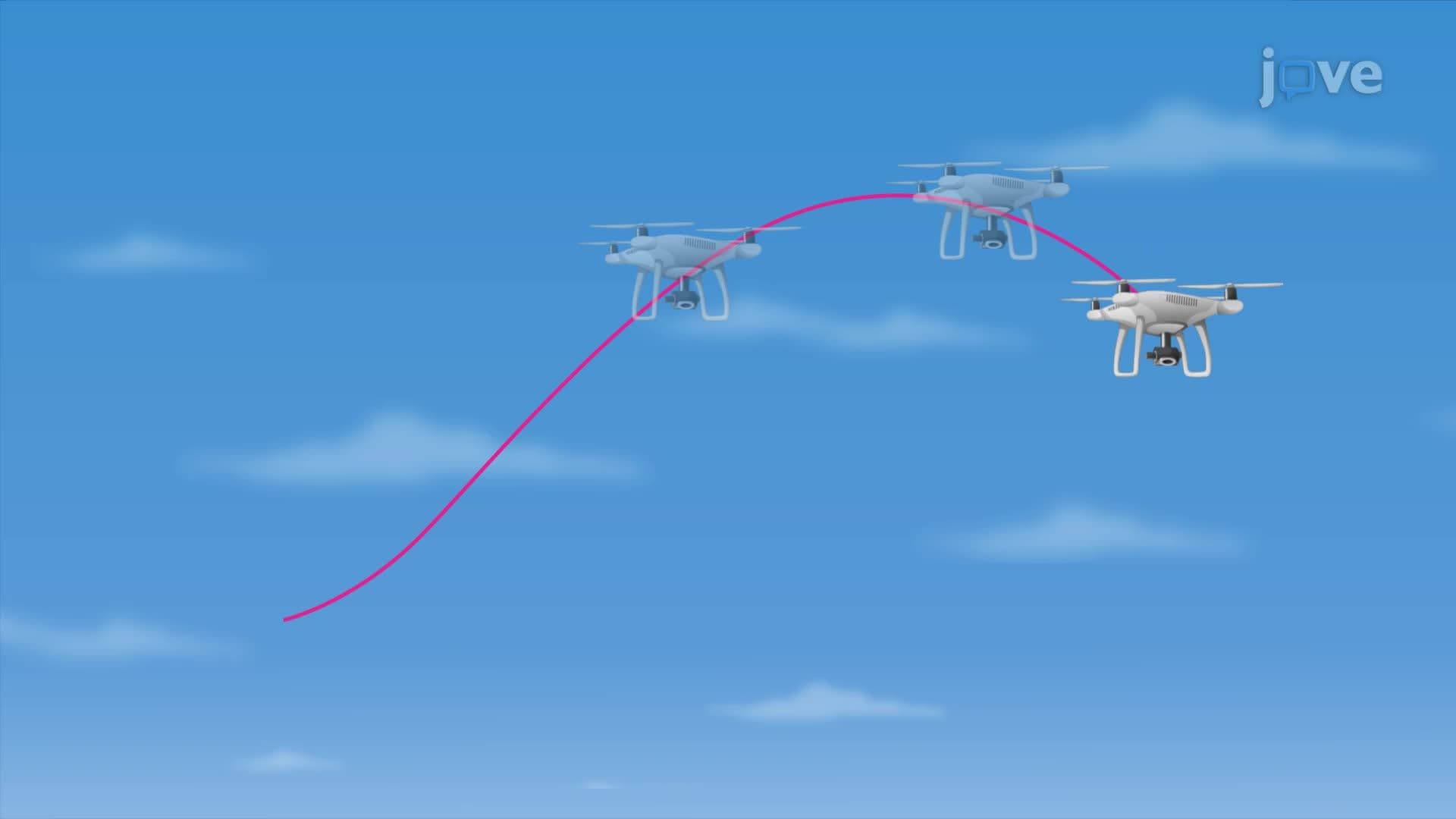

Video Summary: Velocity and Acceleration of Motion in Space
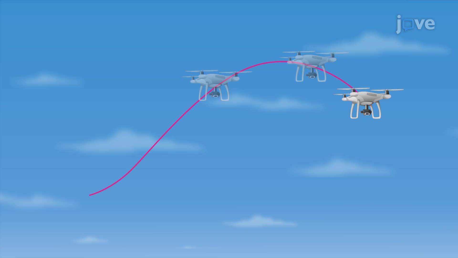
Ever wonder how NASA engineers track a spacecraft's changing speed and direction in three-dimensional space? Velocity and acceleration of motion in space unlocks exactly that, extending calculus concepts to vector-valued functions that model real movement. Using a drone as a relatable example, this lesson shows how derivatives of position vectors reveal instantaneous velocity and acceleration in 3D. Watch the full video on JoVE Coach to master this concept with expert-led visuals and step-by-step explanations.
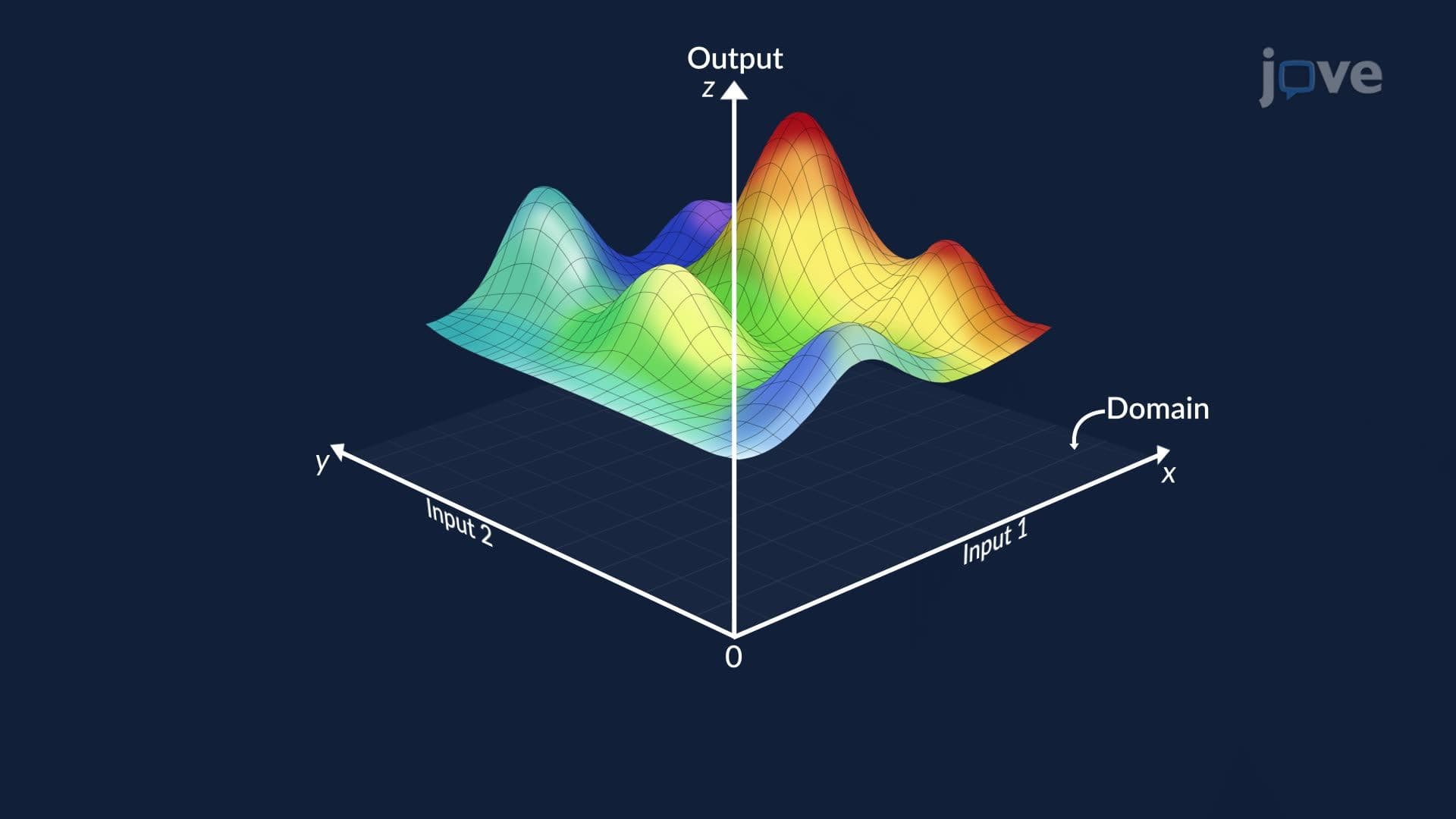
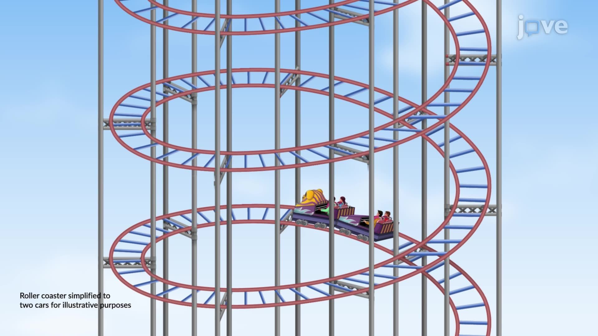
In single-variable calculus, motion is typically studied along a straight line. But real objects, satellites, aircraft, roller coasters, and footballs thrown at an angle, move through three-dimensional space along curved paths. Velocity and acceleration of motion in space is the framework that handles this complexity. By representing position as a vector-valued function r(t) = f(t)i + g(t)j + h(t)k, calculus can be extended naturally to describe motion in full 3D detail. This concept appears prominently in college Calculus III (Multivariable Calculus) courses across US universities and is the foundation for advanced topics in physics and engineering.
The velocity vector is defined as the derivative of the position vector with respect to time: v(t) = r'(t). Because differentiation of vector-valued functions is performed component-by-component, if r(t) = t³i + t²j + 2k, then v(t) = 3t²i + 2tj + 0k. This result is geometrically meaningful, the velocity vector is always tangent to the curve at that instant, which is why it is closely tied to the unit tangent vector T(t) = v(t) / |v(t)|. Speed, a scalar, equals the magnitude |v(t)|, and unlike velocity, it carries no directional information. On AP Calculus BC and college midterms, students are frequently asked to find instantaneous speed at a given time, always remember to compute the magnitude after differentiating.
Acceleration measures how velocity changes over time, so it is the second derivative of position: a(t) = v'(t) = r''(t). Continuing the example above, a(t) = 6ti + 2j. Notice that at t = 1, a(1) = 6i + 2j, which shows the drone accelerating in both the x and y directions simultaneously. This is a key insight: in space, acceleration can change an object's speed, direction, or both, unlike one-dimensional motion where acceleration only affects speed. NASA's Jet Propulsion Laboratory (JPL) uses these exact principles when computing trajectory corrections for deep-space probes, adjusting thruster burns based on continuous recalculation of velocity and acceleration vectors.
Once velocity and acceleration vectors are understood, deeper analysis becomes possible. The acceleration vector can be decomposed into two components: the tangential component of acceleration, which acts along the direction of motion and changes speed, and the normal component of acceleration, which acts perpendicular to motion and changes direction. This decomposition is essential in physics courses when analyzing circular or curved motion. The normal vector (also called the principal unit normal) points toward the center of curvature, while the binormal vector completes a three-dimensional coordinate frame called the TNB frame. Curvature, often written as kappa (κ), measures how sharply a curve bends at any point; it equals the rate of change of the unit tangent vector with respect to arc length. The arc length of a space curve is computed by integrating the speed over an interval: L = integral from a to b of |v(t)| dt. These concepts all appear in Calculus III syllabi at major US universities including MIT, UCLA, and the University of Texas, and are tested on college midterms and finals in both math and engineering physics sequences.
Related Micro-courses