Loading video…

 24 Concepts
 93 views

Video Summary: What are Functions of Two Variables
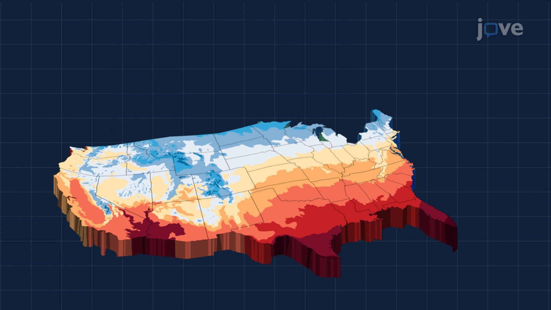
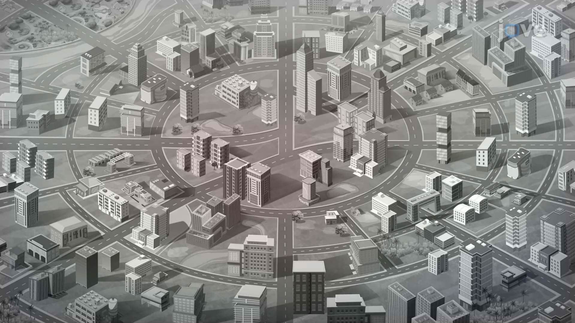
Did you know a city's traffic flow can be modeled as a mathematical surface? Functions of two variables make this possible, a core concept in multivariable calculus where two inputs produce a single output. For instance, traffic density on a US highway depends on both road position and time of day, generating a 3D surface of patterns. Watch the full video on JoVE Coach to master this concept with expert-led visuals and step-by-step explanations.
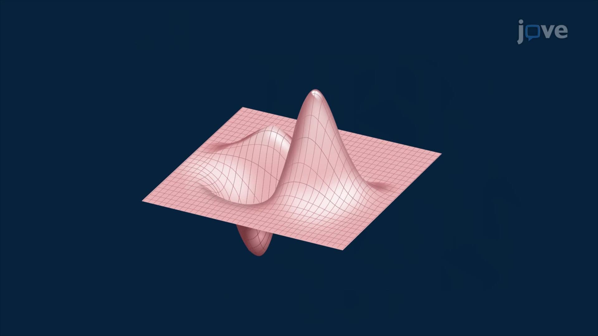
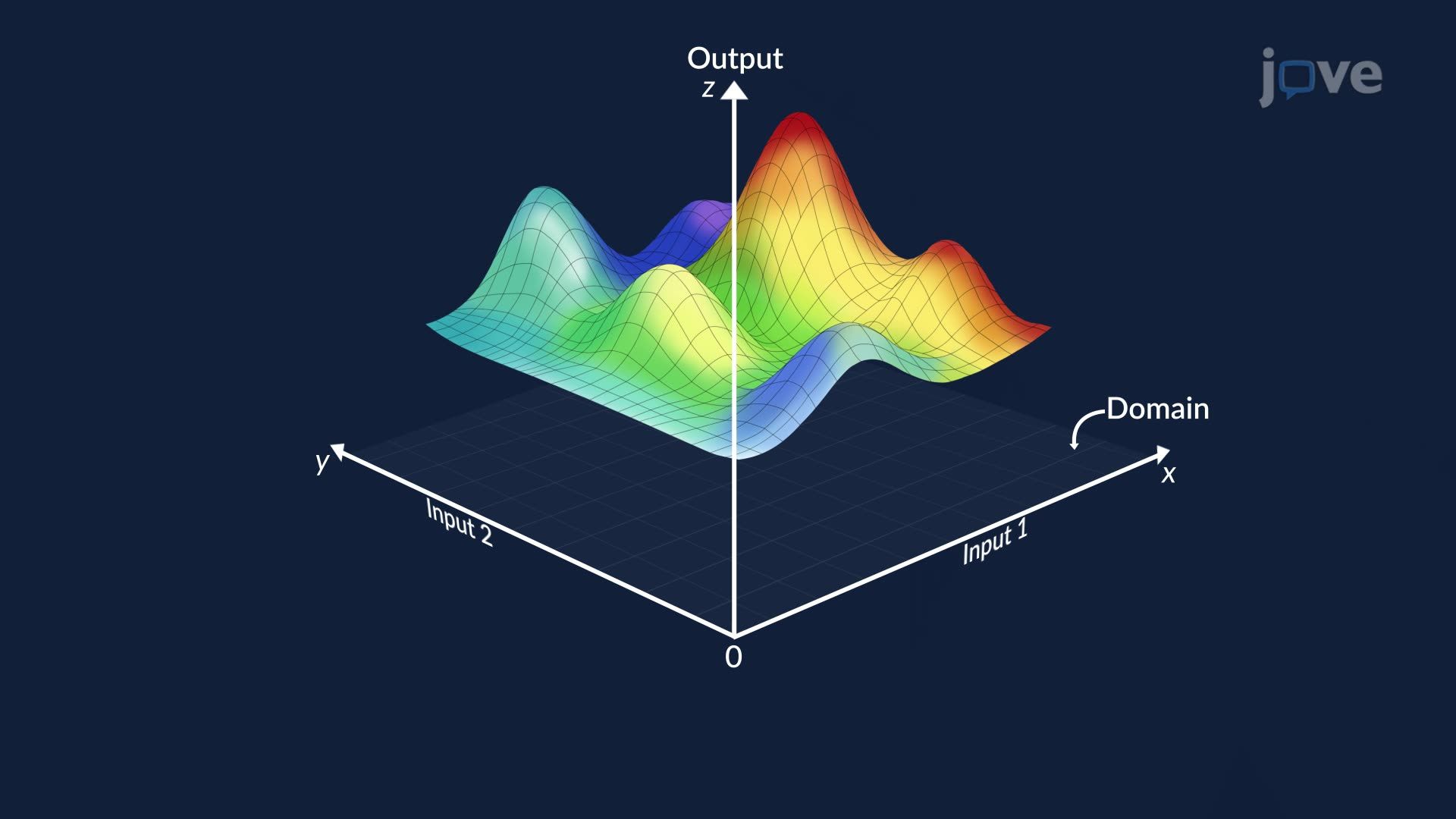
In single-variable calculus, a function takes one input and returns one output, think of graphing y = f(x) as a curve on a flat plane. But most phenomena in the real world are driven by more than one factor at once. Functions of two variables, written as z = f(x, y), extend this idea by accepting two independent inputs and producing a single output. The result isn't a curve; it's a surface stretching through three-dimensional space. This shift from 2D to 3D thinking is the gateway to multivariable calculus, a subject central to college-level STEM curricula across the US.
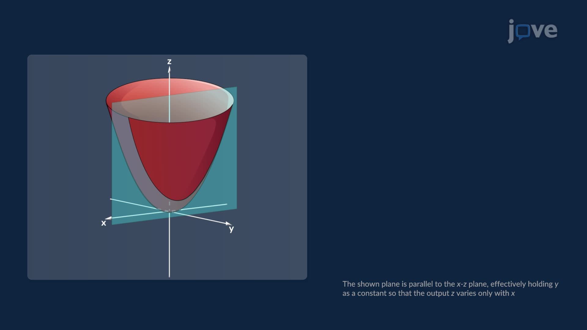
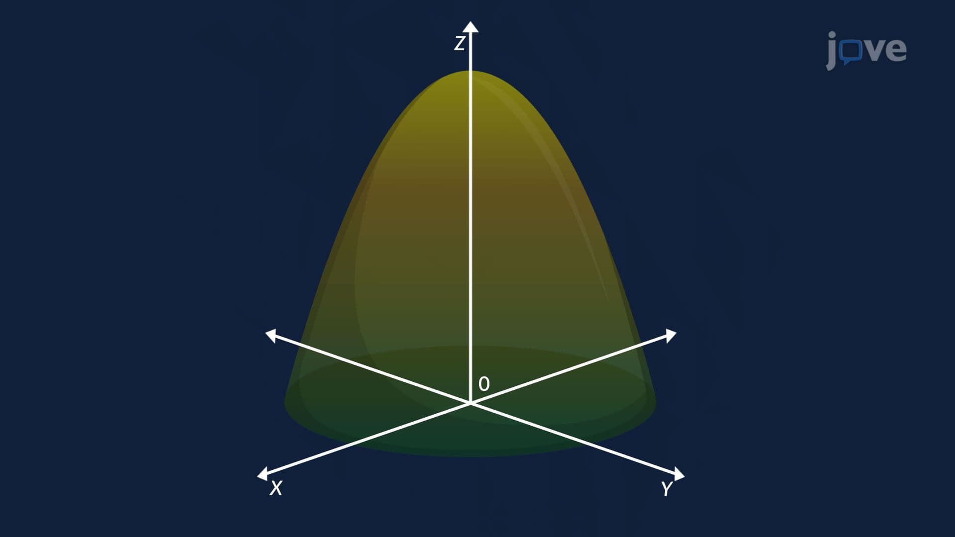
For a function of two variables, the domain is a region in the xy-plane, every valid (x, y) pair that the function can accept. Each point in this region represents a unique combination of inputs. The output, z, is plotted as a vertical height above that point. When you connect all these heights continuously, you build a surface. For example, z = x² + y² produces a bowl-shaped surface called a paraboloid. Visualizing these surfaces, whether by hand or using graphing tools like Desmos 3D or GeoGebra, is a skill heavily tested in college calculus courses and AP Calculus BC extensions.
Consider traffic density on a major corridor like I-95 in the northeastern US. The density D depends on two inputs: position along the road (x, measured in miles from a reference point) and time of day (t, measured in hours). So D = f(x, t) is a genuine function of two variables. As x and t vary, the function's surface rises sharply during morning and evening rush hours and flattens during off-peak periods. Transportation agencies use models like this to optimize signal timing, predict congestion, and plan infrastructure improvements, turning abstract calculus into life-improving engineering decisions.
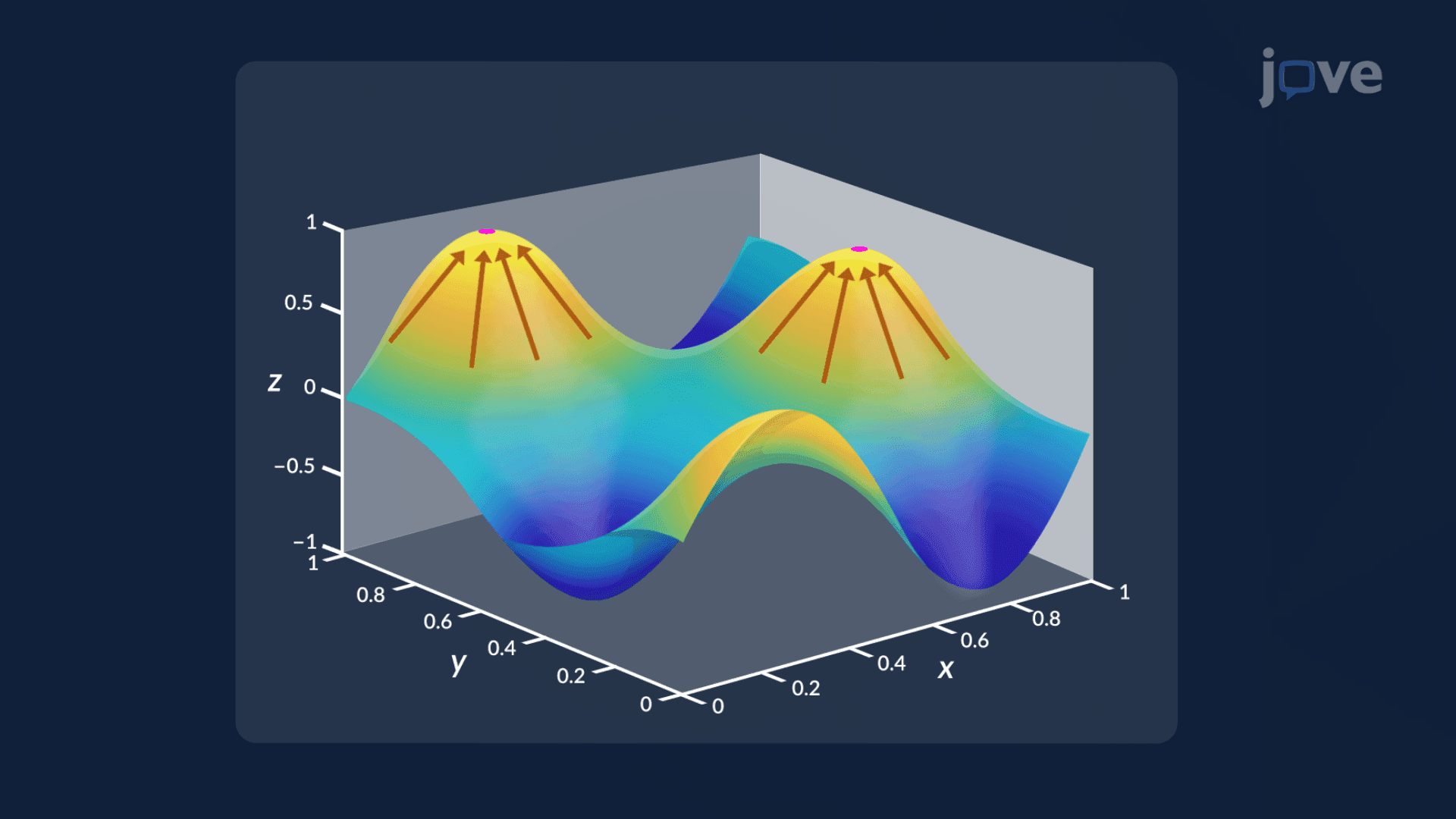
Once you understand the basics of two-variable functions, a powerful toolkit opens up. Partial derivatives measure how z changes when only one variable shifts while the other stays fixed, for instance, how traffic changes with time at a fixed location. The gradient vector combines these partial derivatives and points in the direction of steepest increase on the surface, answering the question: *what is the geometric interpretation of the gradient vector?* From there, directional derivatives generalize this to any direction, while tangent planes provide a flat approximation of the surface at any given point. Exploring higher-order partial derivatives and the chain rule for partial derivatives prepares students for optimization problems, including finding the maximum and minimum values of functions of two variables, a topic that appears on college midterms, Calc III exams, and even portions of the MCAT (physics and quantitative reasoning sections).
Students in AP Calculus BC, college Calculus II/III, or introductory physics and economics courses will encounter two-variable functions regularly. The concept builds critical spatial reasoning, strengthens algebraic manipulation skills, and directly supports topics in thermodynamics, machine learning, and financial modeling. Mastering this foundational idea early, especially the link between the algebraic form z = f(x, y) and its geometric surface, makes every subsequent topic in multivariable calculus significantly more approachable.
Related Micro-courses