Loading video…


 24 Concepts
 92 views

Video Summary: Properties of Limits in Multivariable Calculus Explained
Did you know that the "feels-like" temperature in cities like Phoenix or Houston depends on multiple variables, temperature, humidity, and wind, all changing simultaneously? Understanding properties of limits in multivariable calculus reveals how these combined quantities behave predictably near any given point. The sum law and difference law are foundational tools that make this analysis possible. Watch the full video on JoVE Coach to master this concept with expert-led visuals and step-by-step explanations.
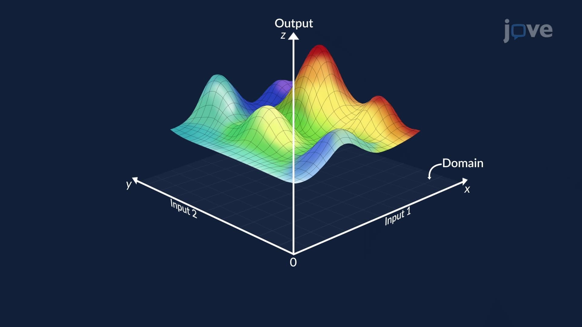
When you move from single-variable calculus to multivariable calculus, limits don't disappear, they get richer. Instead of asking what happens to f(x) as x approaches one value, you now ask what happens to f(x, y) as a point (x, y) approaches a specific location from *any direction*. This added complexity makes it essential to have reliable rules for simplifying these expressions. That's exactly what the properties of limits in multivariable calculus provide.
The sum law states that the limit of a sum of two functions equals the sum of their individual limits, but only when each individual limit exists. In notation: lim[f(x,y) + g(x,y)] = lim f(x,y) + lim g(x,y).
This is enormously useful when dealing with real systems that combine multiple inputs. Consider the National Weather Service's "heat index", the official measure of how hot it feels in US cities when humidity is factored in. If temperature contributes one function T(x, y) and humidity contributes another function H(x, y), the combined perceived heat P(x, y) = T(x, y) + H(x, y) can be analyzed near any location simply by evaluating each limit separately. This decomposition saves time and reduces errors in both academic problems and applied modeling.
Just as important is the difference law, which states that the limit of a difference equals the difference of the individual limits, again provided both limits exist: lim[f(x,y) - g(x,y)] = lim f(x,y) - lim g(x,y).
Returning to the weather example: wind speed lowers the perceived heat. If W(x, y) models the wind-cooling effect, the net perceived heat becomes P(x, y) - W(x, y). The difference law guarantees that as you approach a fixed location, the limit of this net effect equals the limit of P minus the limit of W. This clean separation is what makes multivariable models mathematically tractable.
These limit laws aren't just introductory rules, they underpin everything that follows in multivariable calculus. Partial derivatives, for instance, are defined using limits, and the chain rule for partial derivatives depends on limits behaving consistently when variables change along a path. Similarly, understanding how functions behave near a point is the geometric foundation for tangent planes and the gradient vector. When you later study directional derivatives or ask "What is the geometric interpretation of the gradient vector?", you're building directly on the limit behavior established here.
In AP Calculus BC, limit properties appear throughout the curriculum, though multivariable extensions are more common at the college level in courses like Calculus III (often called Multivariable Calculus). Students in STEM programs at US universities, engineering, physics, economics, encounter these properties in their first or second semester of college calculus. They frequently appear on college midterms and finals in problems involving continuity, differentiability, and optimization, including finding maximum and minimum values of functions of two variables. Mastering the sum and difference laws early creates a confident foundation for all of these topics.
Related Micro-courses