Loading video…

 24 Concepts
 92 views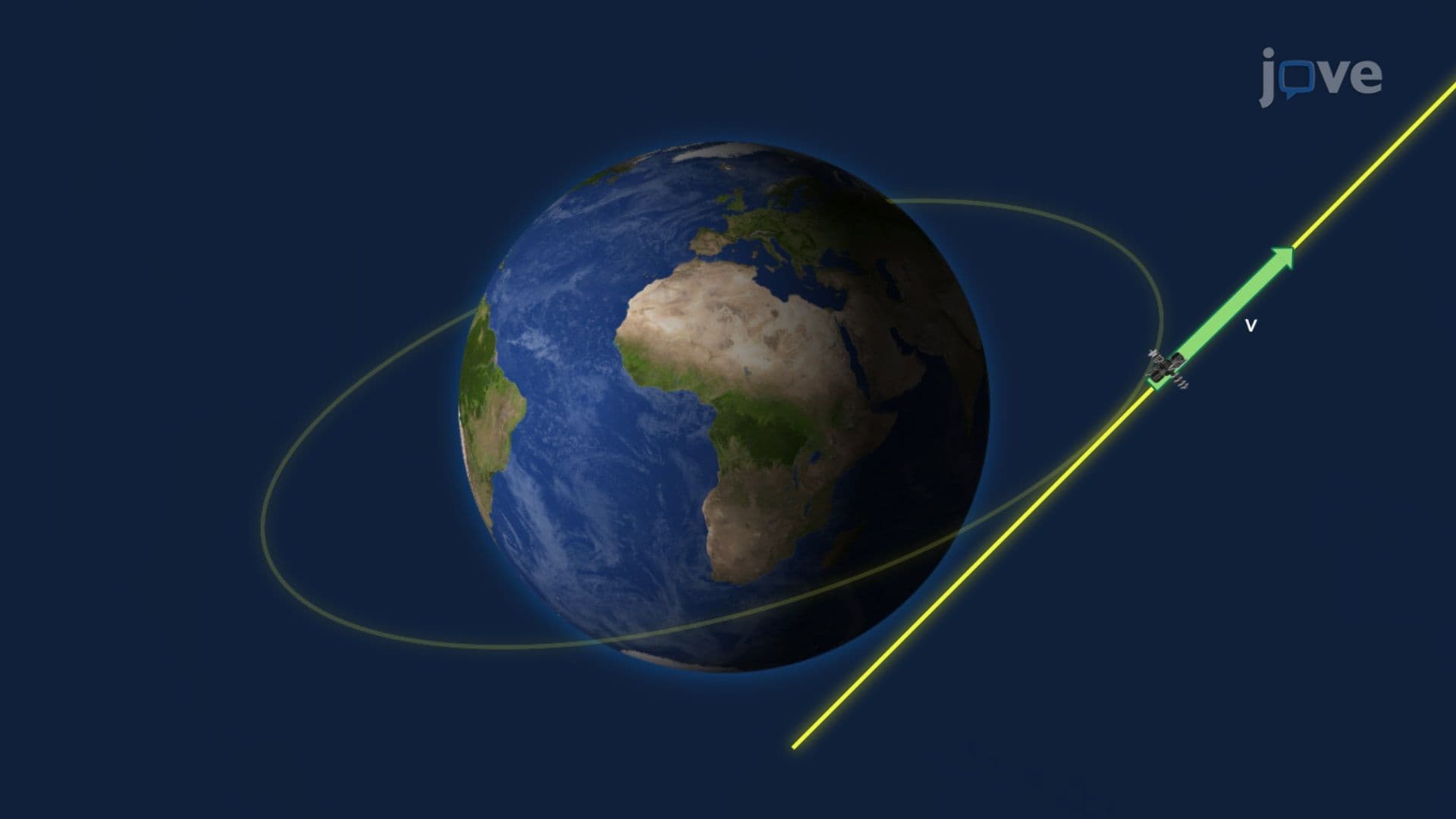

Video Summary: Implicit Differentiation with Partial Derivatives Explained
Ever wonder how NASA engineers calculate a satellite's velocity without ever solving for its exact orbital equation? That's where implicit differentiation with partial derivatives comes in. This powerful multivariable calculus technique lets you find rates of change in equations where y can't easily be isolated, like a satellite's circular orbit described by x² + y² = r². Watch the full video on JoVE Coach to master this concept with expert-led visuals and step-by-step explanations.
In single-variable calculus, you typically differentiate a function written explicitly as y = f(x). But many real-world relationships, from orbital paths to pressure-volume curves in thermodynamics, can't be neatly solved for one variable. Implicit differentiation with partial derivatives is the technique that handles these situations in multivariable calculus. When a relationship is expressed as F(x, y) = 0, and y is implicitly a function of x, this method allows you to compute dy/dx directly without ever isolating y.
The foundation of this method is the chain rule for partial derivatives. When you differentiate both sides of F(x, y) = 0 with respect to x, the chain rule produces two terms: the partial derivative of F with respect to x (written F(x)), times dx/dx, plus the partial derivative of F with respect to y (written F(y)), times dy/dx. Since dx/dx = 1, this simplifies immediately. Rearranging gives the clean implicit differentiation formula:
dy/dx = −F(x) / F(y)
This formula is valid as long as F(y) ≠ 0, a condition tied to the Implicit Function Theorem, a cornerstone result in multivariable calculus taught in courses like Calculus III at universities across the US.
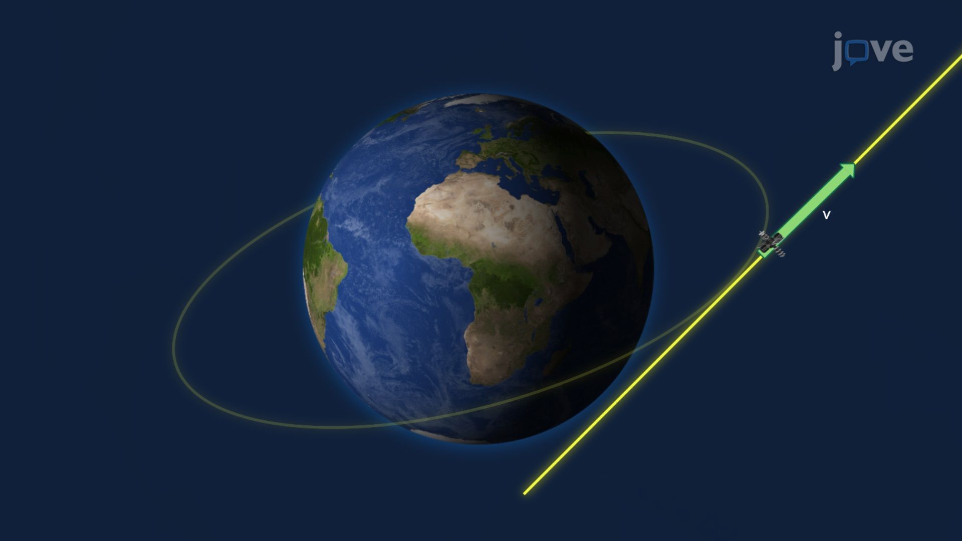
Consider a satellite in circular orbit described by the equation x² + y² = r², where r is the orbital radius. This equation defines y implicitly, solving for y gives two branches (upper and lower orbit), making explicit differentiation awkward. Using the partial derivative approach, F(x) = 2x and F(y) = 2y, so the slope at any point is dy/dx = −x/y. This instantaneous slope defines the velocity vector, the direction the satellite would travel if released from gravitational pull at that exact moment. NASA mission planners and aerospace engineers at institutions like the Jet Propulsion Laboratory (JPL) in Pasadena, California, use exactly this kind of analysis when calculating orbital insertion or escape trajectories.
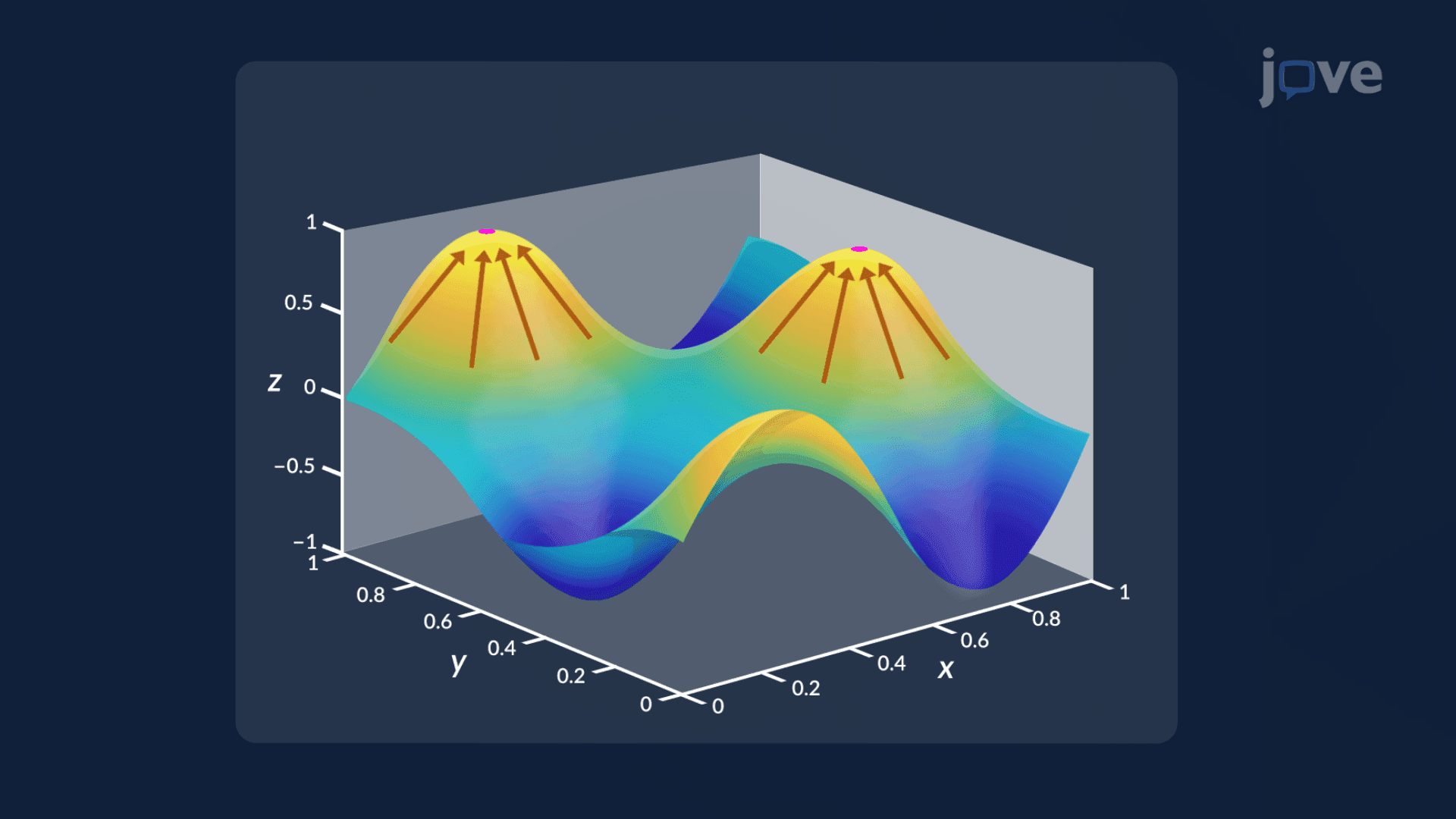
Mastering this technique opens doors to several advanced concepts. The ratio −F(x)/F(y) is directly related to the gradient of a function, the vector ∇F = ⟨F(x), F(y)⟩ always points perpendicular to the level curve F(x, y) = 0. This geometric interpretation underpins tangent planes to surfaces in three dimensions and is essential for understanding directional derivatives. From there, the path leads naturally to analyzing maximum and minimum values of functions of two variables using second-order conditions, topics covered in AP Calculus BC, college Calculus II, and Calculus III courses nationwide.
For AP Calculus BC students, implicit differentiation in single-variable form is a tested skill, and understanding the partial derivative extension prepares students for college-level multivariable courses. College midterms in Calculus III routinely ask students to apply this exact formula to curves like ellipses, hyperbolas, and implicitly defined surfaces. On the MCAT, related reasoning about rates of change appears in physics passages involving circular motion and fluid dynamics. Recognizing when to use implicit differentiation, and correctly identifying when F(y) = 0 makes the formula undefined, is a common source of exam errors that solid conceptual understanding eliminates.
Related Micro-courses