Tangent Planes to Surfaces

• Understand what tangent planes to surfaces are and how they extend the single-variable idea of a tangent line into three-dimensional space
• Identify how partial derivatives define the slopes of cross-sectional curves that together determine a unique tangent plane at a given point
• Apply the tangent plane equation to linearly approximate a surface near a chosen point, simplifying complex multivariable analysis
• Recognize the connection between tangent planes, the gradient vector, and directional derivatives in multivariable calculus
• Analyze how changes in x and y independently contribute to changes in z through the linear structure of the tangent plane equation
• Compare the behavior of a surface at a point with its tangent plane approximation to evaluate accuracy near and away from that point
• Explore how tangent planes relate to finding maximum and minimum values of functions of two variables and identifying local extrema
• Evaluate real-world scenarios, such as terrain modeling or surface design, where tangent plane approximations are used to make complex shapes manageable

What Are Tangent Planes to Surfaces? A Foundation in Multivariable Calculus

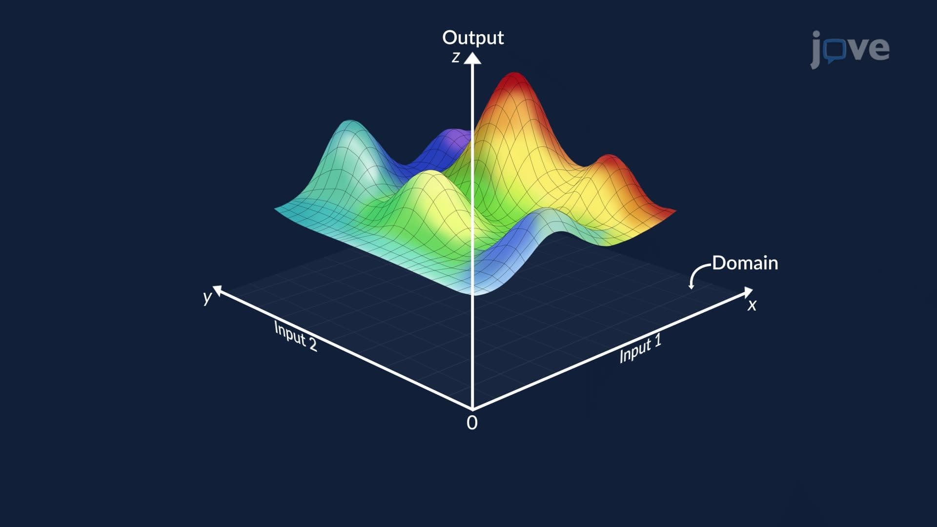
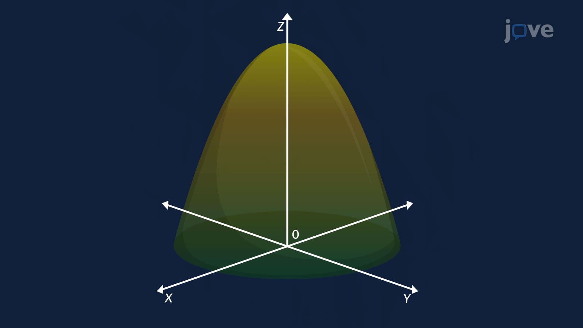
In single-variable calculus, a tangent line touches a curve at one point and approximates it locally. Tangent planes to surfaces extend this idea into three dimensions. When you have a surface where height z depends on two variables x and y, written as z = F(x, y), you need more than one slope to describe local behavior. You need a flat plane that best fits the surface at a chosen point. That plane is the tangent plane, and it is one of the most important tools in multivariable calculus.

How Partial Derivatives Build the Tangent Plane

To construct the tangent plane at a point, two cross-sectional curves are examined. One curve is formed by slicing the surface parallel to the xz-plane (holding y constant), and the other by slicing parallel to the yz-plane (holding x constant). Each curve has a tangent line at the chosen point. The slopes of these tangent lines are the partial derivatives: dF/dx and dF/dy, evaluated at that point.

The tangent plane equation combines both slopes linearly:

z − z₀ = (dF/dx)(x − x₀) + (dF/dy)(y − y₀)

Here, (x₀, y₀, z₀) is the point of tangency. The coefficients, the partial derivatives, tell you exactly how sensitive the surface height is to small changes in each direction. This structure connects directly to the gradient vector, which packages both partial derivatives together as ∇F = ⟨dF/dx, dF/dy⟩.

Linear Approximation: Why Tangent Planes Matter in Practice

Near the point of tangency, the tangent plane serves as a linear approximation of the surface. This is sometimes called the local linearization. Just as zooming into a curved road makes it look straight, zooming into a curved 3D surface makes it look flat, and the tangent plane captures that flat approximation mathematically.

This idea is critical in engineering and data science. For example, the US Geological Survey (USGS) uses surface approximations when modeling terrain elevation for flood prediction and land-use planning. In robotics programs at universities like MIT and Stanford, tangent plane approximations help autonomous systems navigate uneven terrain in real time by treating small surface patches as flat.

Connections to Broader Calculus Concepts and Exam Relevance

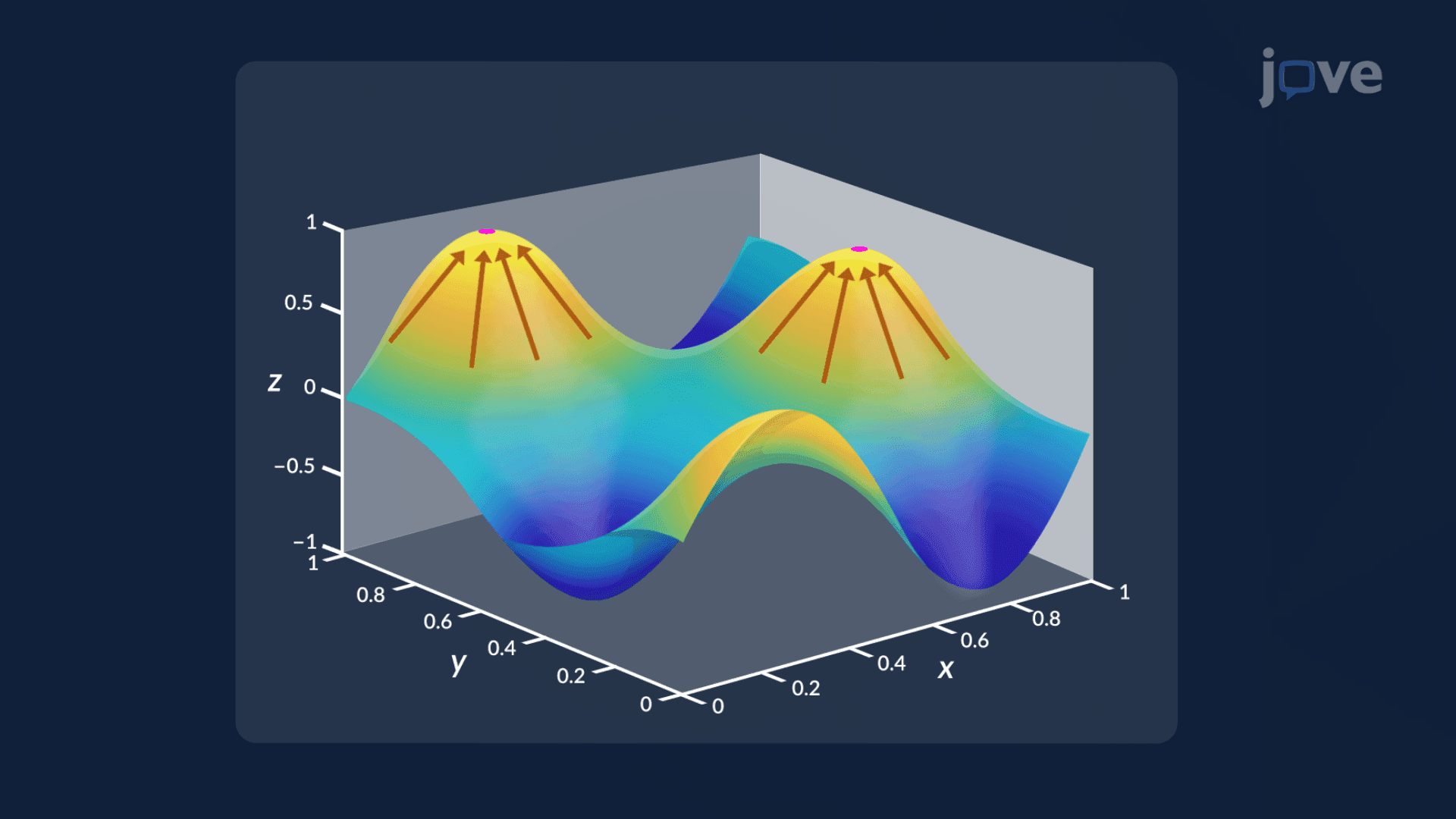
Tangent planes are a gateway concept. Once you understand them, directional derivatives become natural, they measure the rate of change of F(x, y) in any direction, not just along the axes. The gradient vector points in the direction of steepest ascent on the surface, which is geometrically perpendicular to the tangent plane's level curve at that point.

In college-level calculus courses, typically Calculus III or Multivariable Calculus, tangent planes appear in units on differentiation, linear approximation, and optimization. They are prerequisite knowledge for understanding higher-order partial derivatives and the second derivative test used to classify maximum and minimum values of functions of two variables. On college midterms and finals, students are commonly asked to write the tangent plane equation at a specific point, use it to estimate nearby values, or connect it to gradient and directional derivative problems.

Understanding tangent planes to surfaces also strengthens conceptual reasoning tested in STEM courses at the undergraduate level, particularly in physics, engineering, and economics courses that use multivariable models extensively.