Loading video…

 24 Concepts
 92 views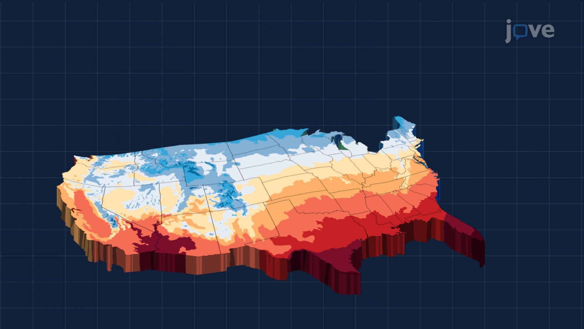

Video Summary: What are Graphs of Two Variable Functions
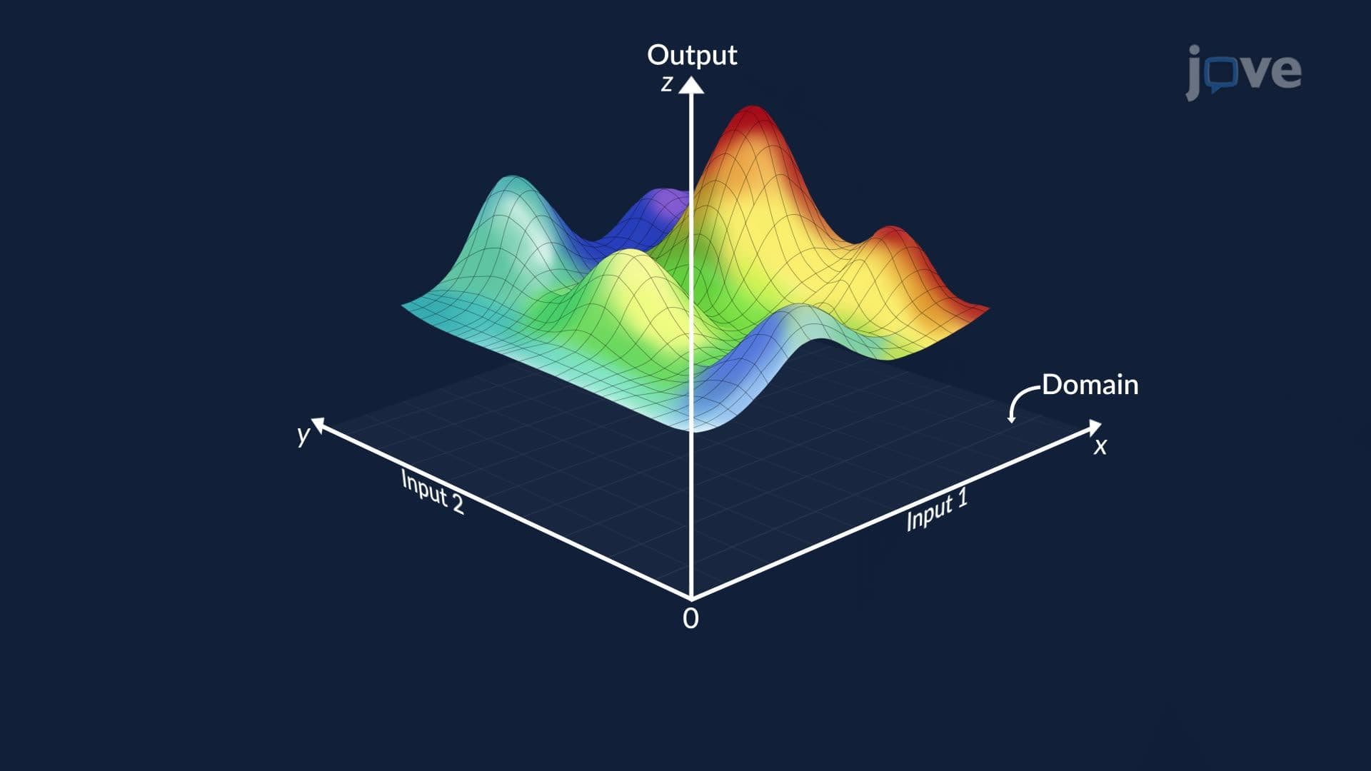
Ever wonder how meteorologists map temperatures across the entire United States at once? Graphs of two-variable functions make that possible. This concept, sometimes called graphs of two-variable functions basics, uses two inputs like longitude and latitude to produce a single output, such as temperature, plotted as a 3D surface described by z = f(x, y). Watch the full video on JoVE Coach to master this concept with expert-led visuals and step-by-step explanations.
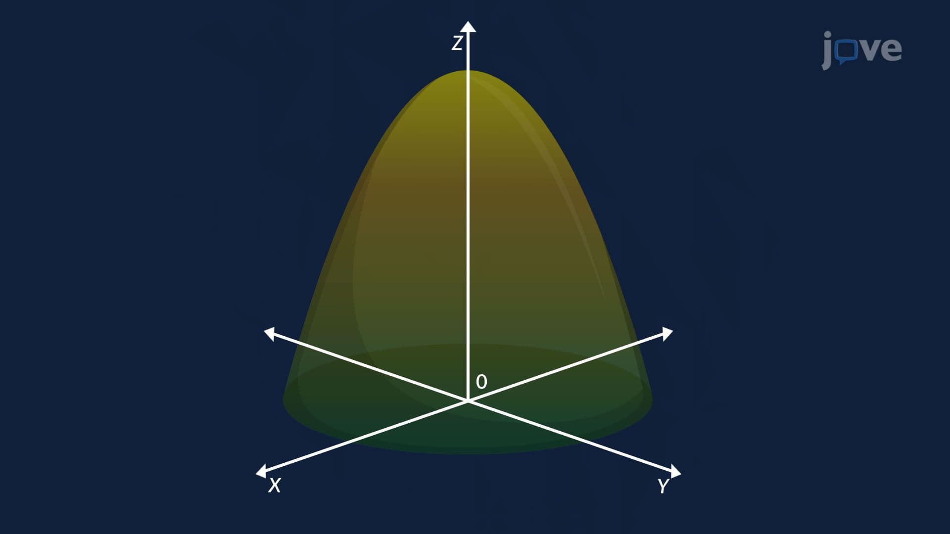
A graph of a two-variable function is a three-dimensional surface that shows how one output value depends on two independent input variables. Written as z = f(x, y), this type of function takes an ordered pair (x, y) as its input and produces a single real number z as its output. That output is plotted along a vertical axis, and when all such points are connected, they form a smooth, continuous surface floating in 3D space. This is the natural extension of the familiar y = f(x) curve from algebra into the world of multivariable calculus.
In a standard single-variable function, you move along one number line (the x-axis) and trace a curve on a flat plane. With two-variable functions, you move across an entire flat grid, defined by both x and y, and the output z rises and falls above that grid like terrain on a topographic map. Peaks on the surface represent local maximum values, valleys represent local minimum values, and flat regions indicate where the function levels off. Developing this geometric intuition is critical for understanding tangent planes, directional derivatives, and the gradient of a function, all core topics in college-level calculus courses such as Calculus III (Multivariable Calculus).
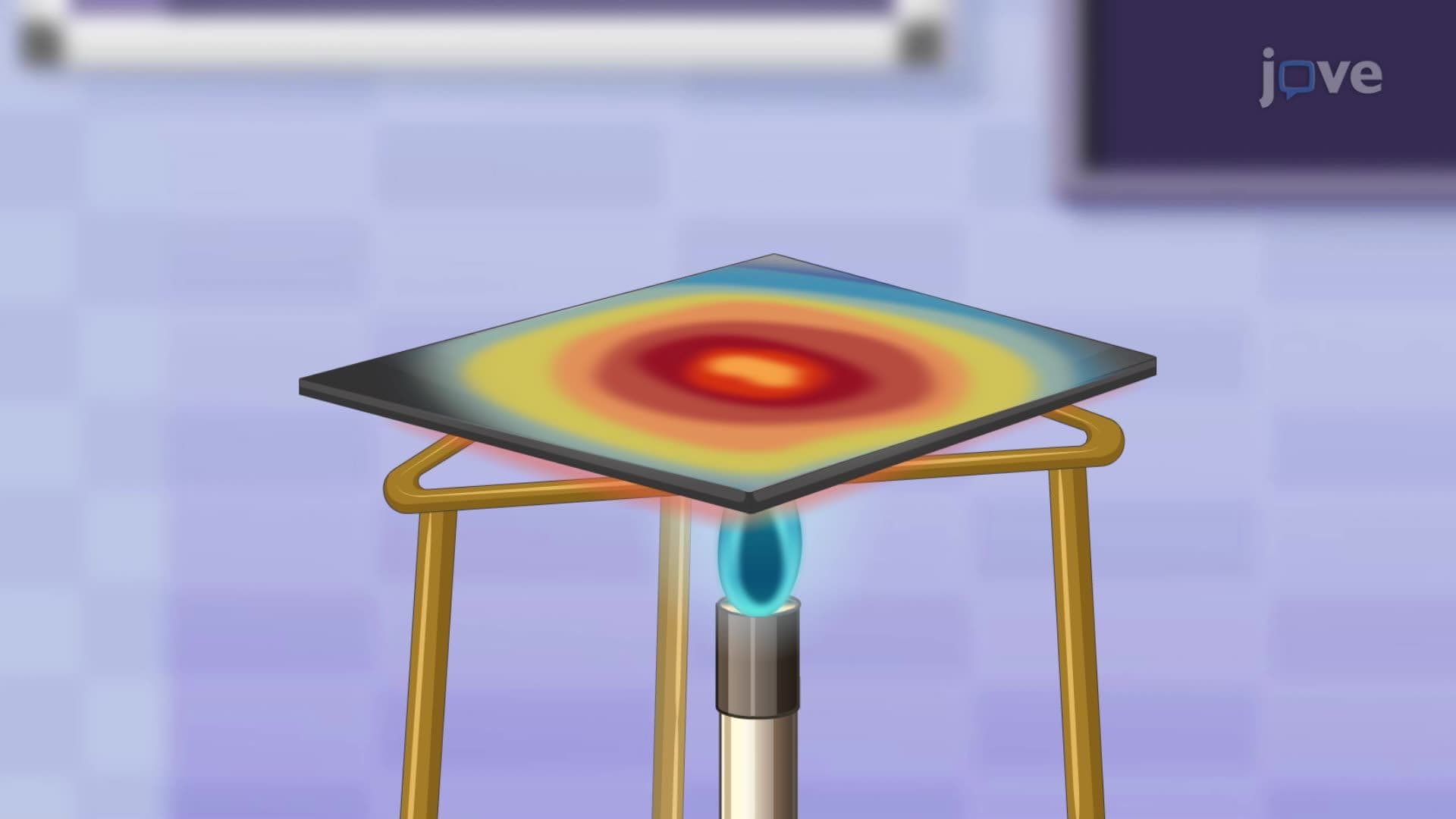
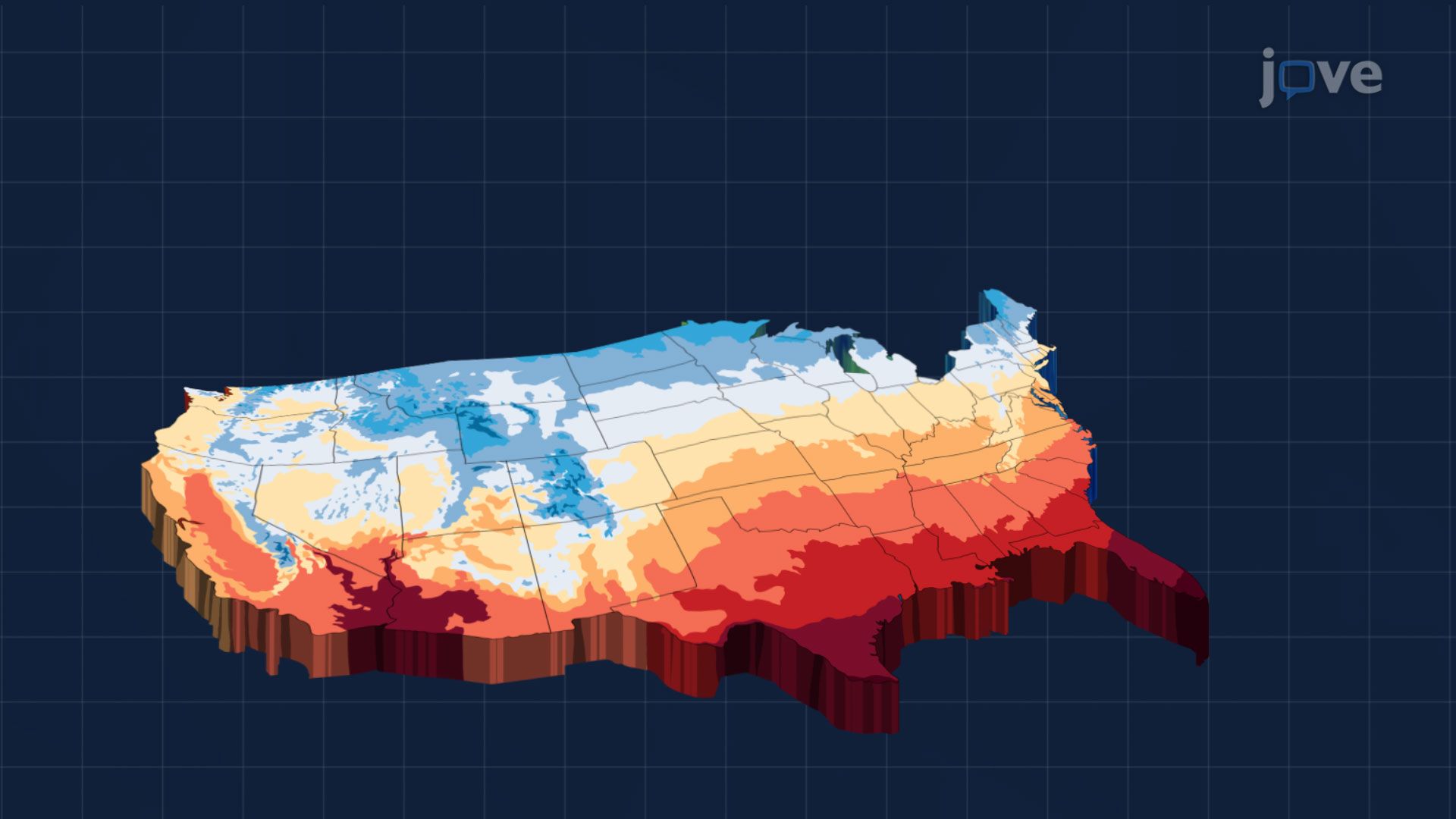
One of the most accessible examples is a US weather map. Longitude and latitude serve as the x and y inputs, while temperature at each location is the z output. The resulting 3D surface visually captures how temperature climbs in the South and dips in the North during winter. Beyond weather, two-variable functions appear throughout science and industry: civil engineers at firms like the US Army Corps of Engineers model terrain elevation using z = f(x, y); economists model cost surfaces where x represents labor and y represents materials; and biomedical researchers at institutions like the NIH use multivariable functions to model drug concentration across tissue regions. These practical applications make the concept directly relevant in AP Calculus BC coursework, college STEM programs, and even MCAT preparation for pre-med students studying biological systems.
Understanding graphs of two-variable functions is the essential first step before tackling more advanced ideas in multivariable calculus. Once you can visualize a 3D surface, the concept of a partial derivative becomes intuitive, it simply measures the slope of the surface in one direction while holding the other input constant. From there, higher-order partial derivatives describe how those slopes themselves change, while the gradient vector points in the direction of steepest ascent on the surface. The chain rule for partial derivatives allows you to handle composite functions across multiple variables. And ultimately, identifying local extrema of a multivariable function, the peaks and valleys of the surface, becomes a matter of finding where the gradient equals zero and applying the second derivative test. Mastering the graph is the geometric foundation that makes all of these algebraic tools meaningful.
Related Micro-courses