Loading video…

 24 Concepts
 92 views

Video Summary: Local Maximum and Minimum Values Explained
What if 12 square meters of cardboard could help you crack one of calculus's most powerful ideas? Local maximum and minimum values, the foundation of optimization in multivariable calculus, describe points on a surface where a function peaks or bottoms out relative to nearby points. Finding these extrema in a real box-volume problem means setting partial derivatives to zero and solving for critical points. Watch the full video on JoVE Coach to master this concept with expert-led visuals and step-by-step explanations.
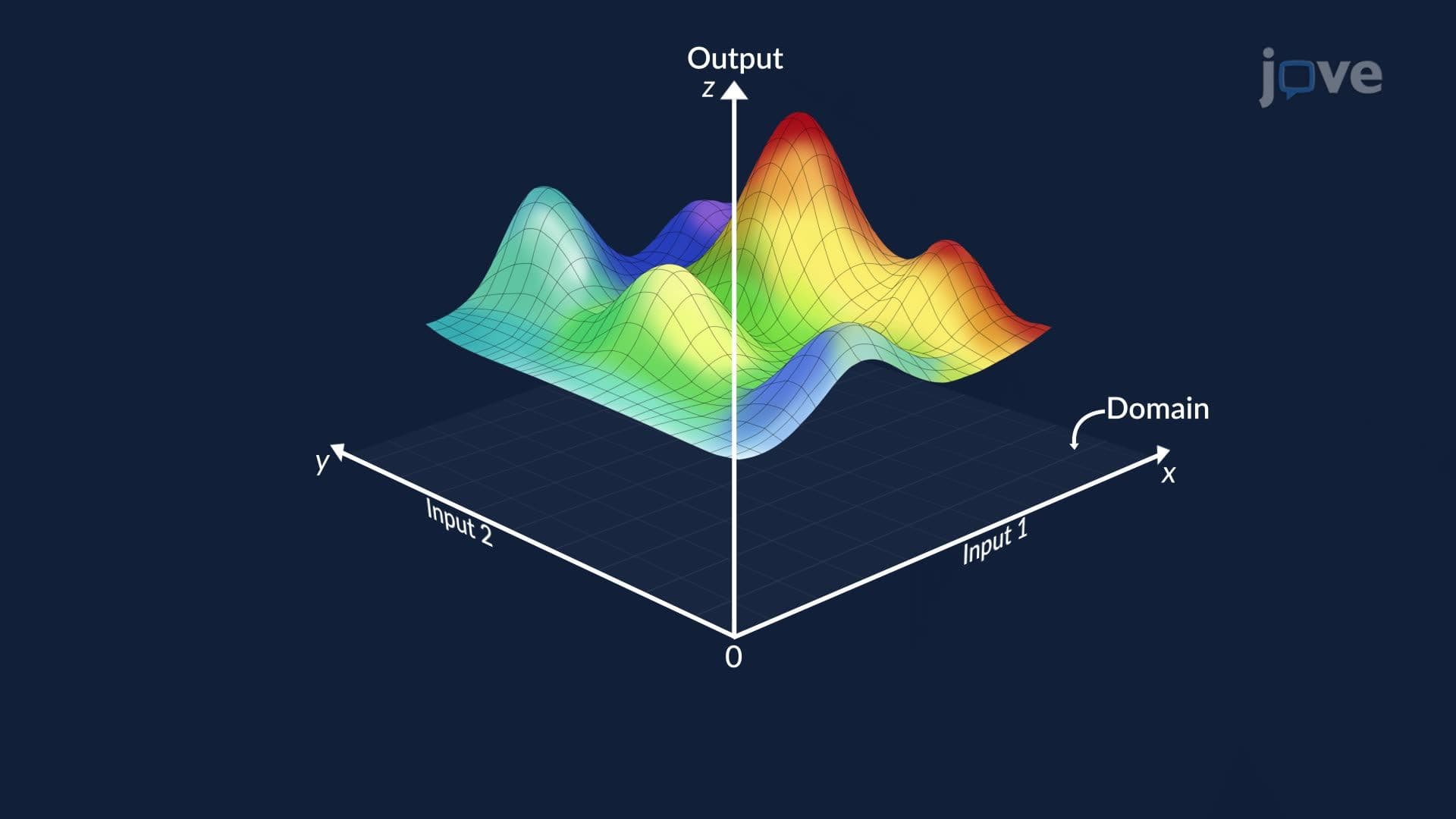
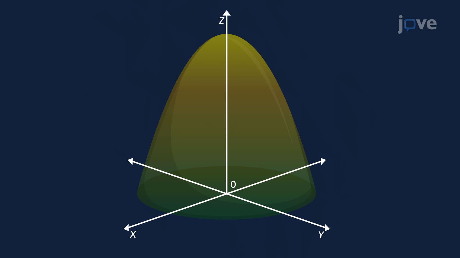
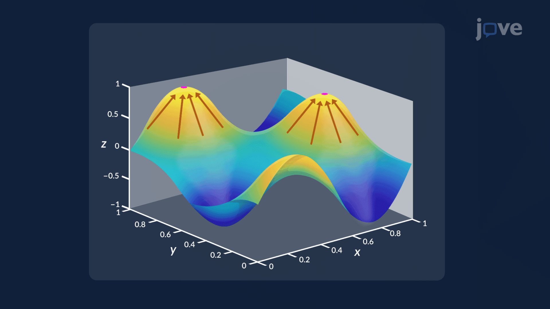
In single-variable calculus, finding where a function rises to a peak or dips to a valley is a familiar task. But in multivariable calculus, a cornerstone of college-level STEM courses across the US, functions depend on two or more variables simultaneously, and their graphs form three-dimensional surfaces. Local maximum and minimum values describe the "hilltops" and "valleys" on these surfaces: points where the function value is higher or lower than every other point immediately surrounding it. Mastering this concept is essential for AP Calculus BC students exploring optimization and for undergraduates in Calculus III courses at universities nationwide.
A critical point of a two-variable function F(x, y) occurs where both the partial derivative of F with respect to x and the partial derivative of F with respect to y equal zero simultaneously. Geometrically, this means the tangent plane at that point is perfectly horizontal, the surface is momentarily "flat," neither rising nor falling in any direction. This is directly analogous to setting a single derivative to zero in one-variable calculus. Not every critical point is a local extremum, however, some are saddle points, where the surface curves upward in one direction and downward in another. Distinguishing between these cases typically requires the Second Derivative Test for functions of two variables, which uses higher-order partial derivatives to classify the critical point.
The gradient of a function is a vector formed by its partial derivatives: it points in the direction of steepest ascent on the surface. At a critical point, the gradient equals zero, there is no direction of ascent or descent. Understanding the gradient ties directly into directional derivatives, which measure how fast a function changes in any chosen direction. When all directional derivatives equal zero at a point, the surface is locally flat, confirming a critical point. This geometric interpretation of the gradient vector is a key exam topic in college Calculus III courses and appears in multivariable optimization problems on college midterms and finals across the US.
One of the most classic US calculus textbook problems involves maximizing the volume of an open-top box built from a fixed amount of material, say, 12 square meters of cardboard. The volume V depends on length x, width y, and height z, but the surface-area constraint ties all three variables together. By expressing z as a function of x and y using the constraint, the problem reduces to maximizing a two-variable function V(x, y). Setting both partial derivatives, V on x and V on y, equal to zero and solving the system of equations identifies the critical point. Substituting those dimensions back into the volume formula gives the maximum volume. This type of constrained optimization problem appears frequently in AP Calculus, college Calculus II and III courses, and even in engineering design curricula at US universities. It builds intuition for more advanced techniques like Lagrange multipliers, which students typically encounter in later multivariable calculus units.
Related Micro-courses