Loading video…

 19 Concepts
 95 views

Video Summary: What are Vector Fields
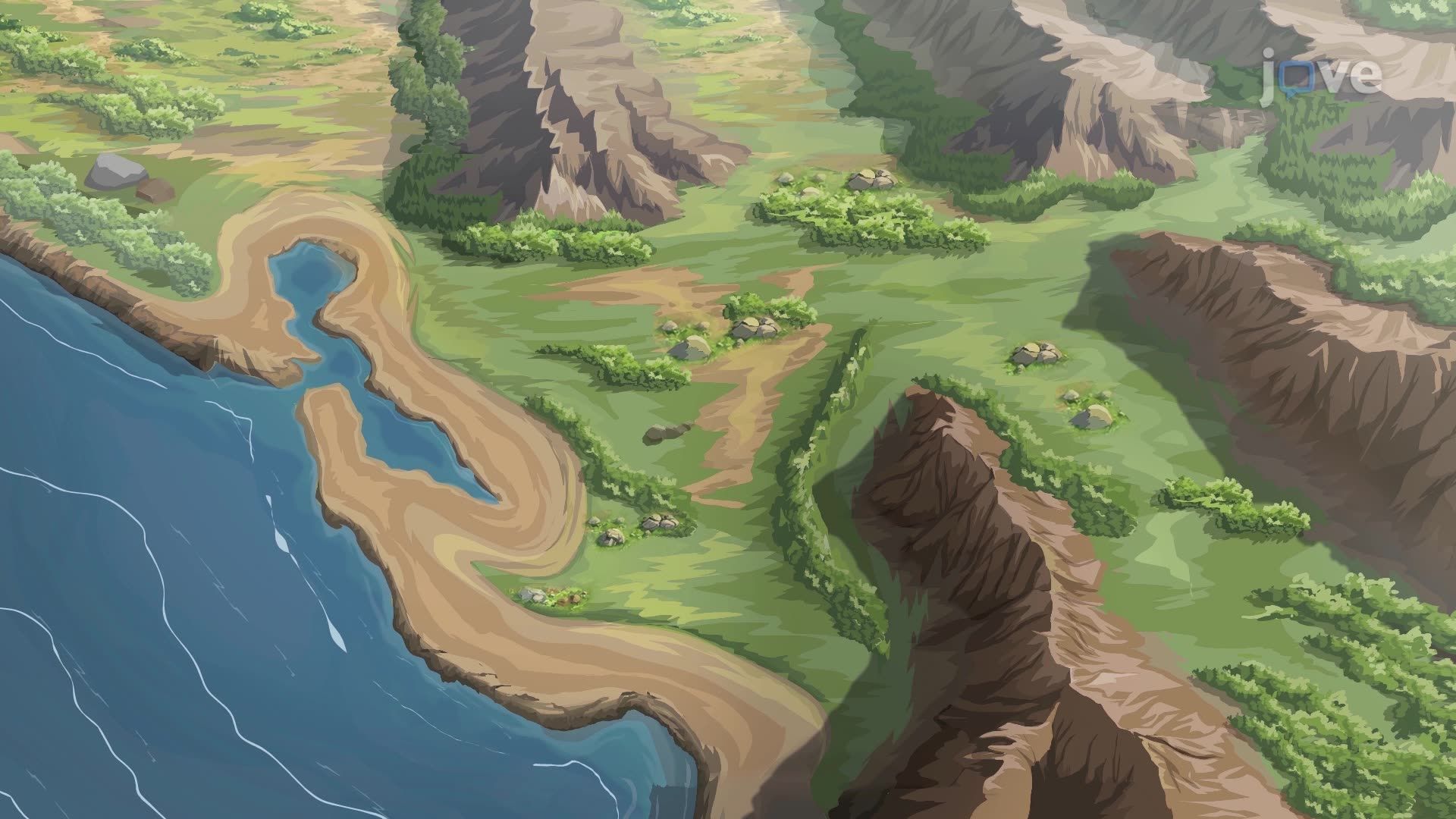
Did you know wind over the San Francisco Bay moves at a different speed and direction at every single location? Vector fields are the mathematical tool that captures exactly this kind of behavior. A vector field assigns an arrow, with both direction and magnitude, to every point in space, making invisible forces like wind, gravity, and fluid flow visible and measurable. Watch the full video on JoVE Coach to master this concept with expert-led visuals and step-by-step explanations.
A vector field is one of the most powerful ideas in multivariable calculus. Unlike a scalar field, which assigns a single number (like temperature) to each point, a vector field assigns both a magnitude and a direction to every point in a region. Formally, a two-dimensional vector field is defined by a function F(x, y) = ⟨P(x, y), Q(x, y)⟩, where P and Q are the component functions that govern horizontal and vertical behavior, respectively. Three-dimensional vector fields add a third component, R(x, y, z), extending this idea into full space.
The behavior of a vector field is entirely controlled by its components. If P(x, y) = 0 and Q(x, y) = 3, every arrow points straight up with equal length, a perfectly uniform field, like a steady northward wind across an open plain. But when Q depends on x, say Q(x, y) = x, arrows grow longer as you move right, reflecting increasing magnitude. This component-by-component analysis is the primary strategy students use to sketch and interpret vector fields without a graphing tool, making it an essential skill on college midterms in Calculus III and Multivariable Calculus courses at universities like MIT OpenCourseWare-aligned programs across the US.
Drawing a vector field means placing arrows at sampled coordinate points, with each arrow's length representing magnitude and its orientation showing direction. Over a map of the San Francisco Bay, for instance, arrows might be short and swirling near the shoreline, reflecting turbulence, but long and consistent over open water, where wind flows freely. This visual representation isn't just intuitive; it's a testable skill. AP Calculus BC students and college undergraduates are frequently asked to match vector field equations to their graphical plots, or to describe the behavior of a given field from its formula alone.
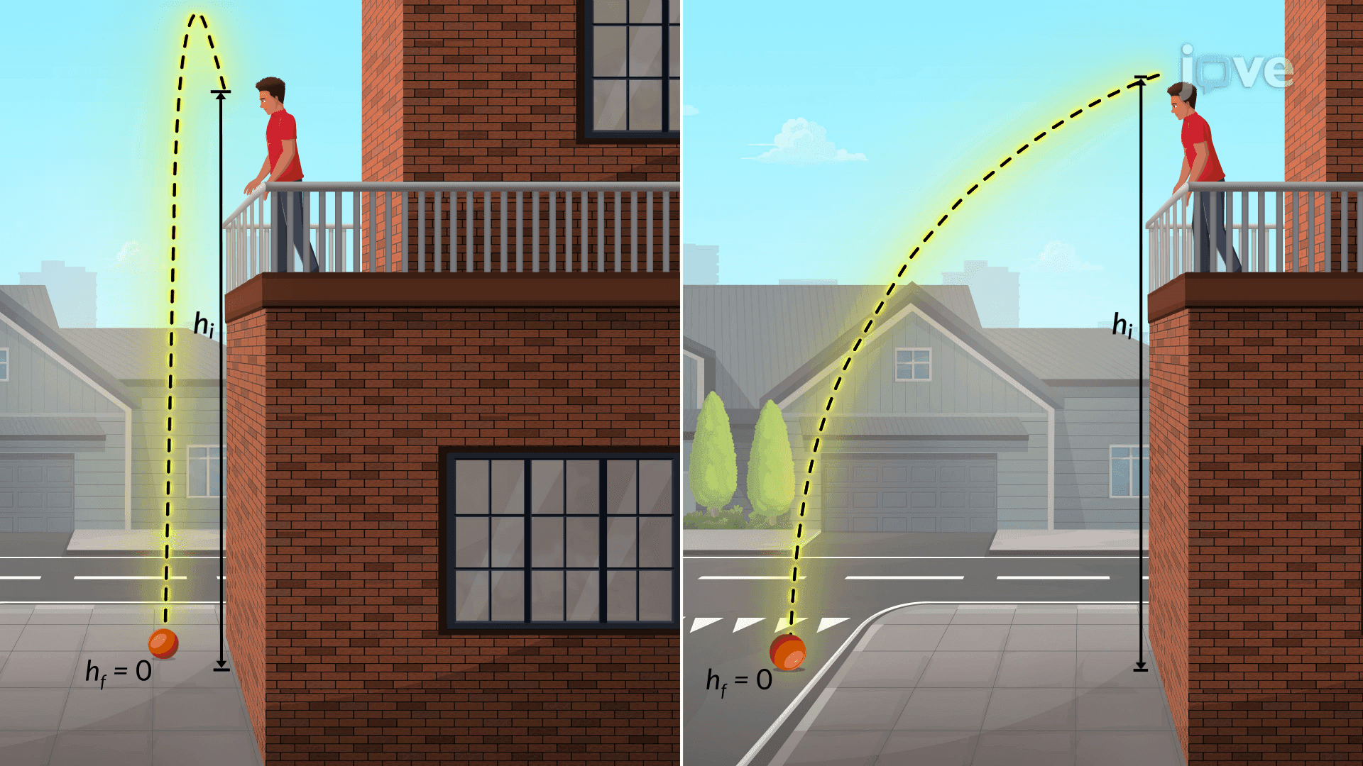
Vector fields are the gateway to some of the most important theorems in mathematics. Line integrals measure work done by a vector field along a curve, critical in physics problems involving force and displacement. Surface integrals extend this to three dimensions. Green's theorem links a line integral around a closed curve to a double integral over the region it encloses, while Stokes' theorem generalizes this relationship to three-dimensional surfaces using curl. The divergence theorem connects the flow of a vector field out of a closed surface to the behavior of its divergence inside. A conservative vector field is a special case where the field is the gradient of some scalar potential function, meaning the line integral between two points is path-independent, a concept central to physics courses, engineering programs, and AP Physics C: Mechanics alike.
Understanding what the physical meaning of divergence is, whether a field is "spreading out" or "converging" at a point, transforms abstract math into real tools used by meteorologists, electrical engineers, and aerospace designers across the United States every day.
Related Micro-courses