Loading video…

 19 Concepts
 95 views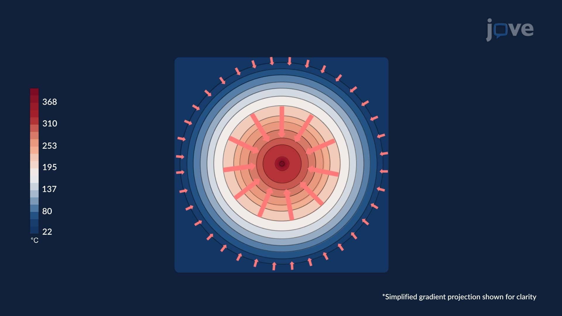

Video Summary: What are Gradient Fields
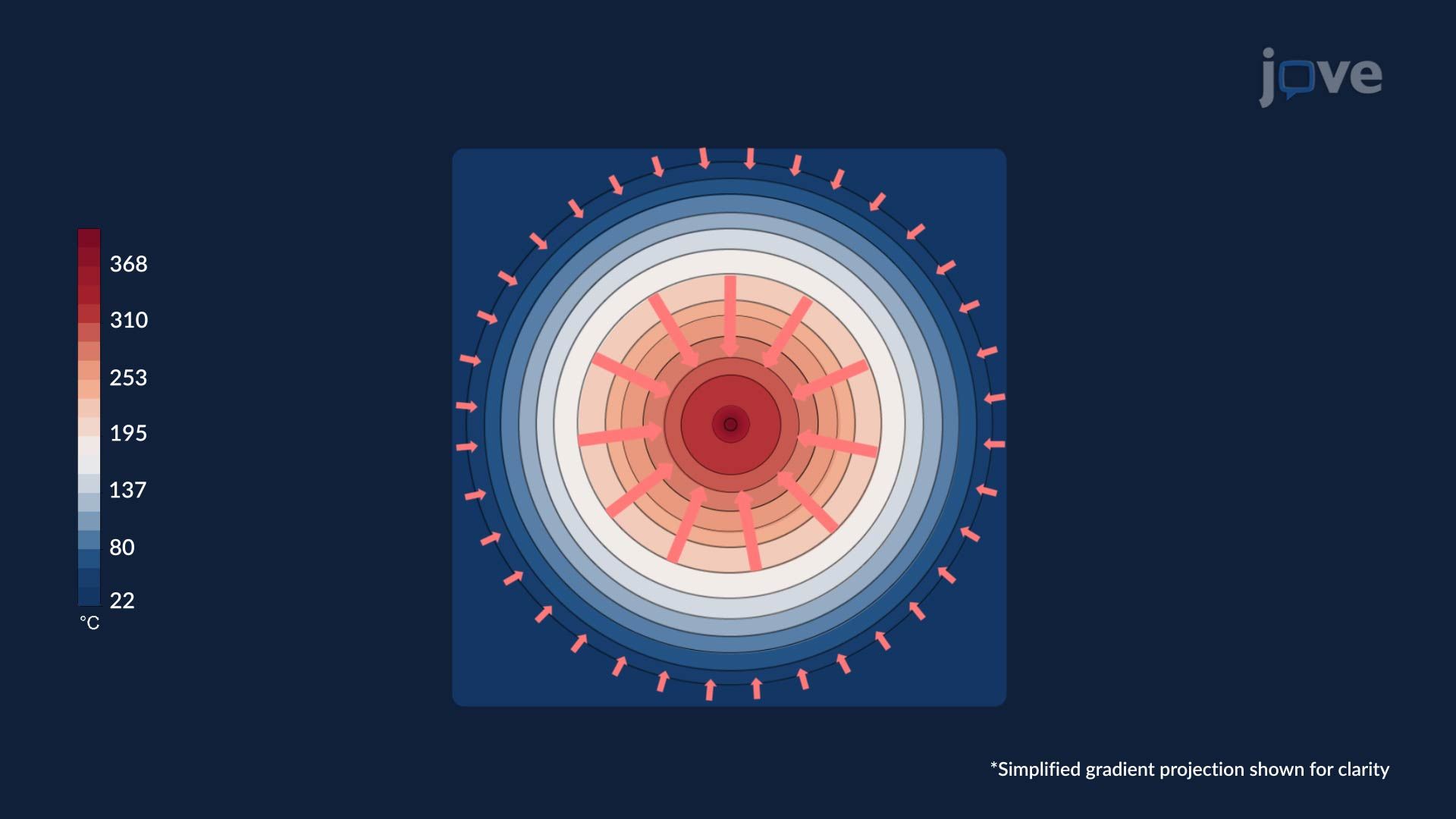
Did you know that engineers at NASA use gradient fields to detect dangerous heat buildup on spacecraft surfaces? Gradient fields basics explain how temperature, pressure, or elevation change across a region, and *what are gradient fields* becomes clear when you picture a heated metal plate: the gradient points toward the steepest temperature rise, always perpendicular to the isotherms. Watch the full video on JoVE Coach to master this concept with expert-led visuals and step-by-step explanations.
Gradient fields are one of the most powerful and intuitive ideas in multivariable calculus. At their core, they answer a simple question: if a quantity like temperature, altitude, or electric potential varies across space, in which direction does it change fastest, and by how much? The answer is the gradient, a vector field built from the partial derivatives of a scalar function. Understanding gradient fields unlocks a chain of deeper concepts in vector calculus, from conservative vector fields and line integrals to Stokes' theorem and the divergence theorem.
A scalar field assigns a single numerical value to every point in space. Temperature across a room, elevation across a landscape, or air pressure across a weather map are all scalar fields. The gradient transforms that scalar field into a vector field, at each point, it produces a vector pointing in the direction of greatest increase, with a magnitude equal to the rate of that increase.
Mathematically, for a function f(x, y), the gradient is written as:
grad f = (∂f/∂x, ∂f/∂y)
Each component is a partial derivative, it captures how f changes when only one variable shifts while the others stay fixed. In three dimensions, a third component (∂f/∂z) is added. This structure is what students encounter in AP Calculus BC extensions, college Calculus III courses, and physics-based courses like electricity and magnetism.
One of the most visually striking properties of a gradient field is its geometric relationship to level curves (or contour lines). A level curve connects all points where the scalar field has the same value, think of elevation contours on a USGS topographic map or isotherms on a National Weather Service temperature map.
The gradient vector at any point is always perpendicular (orthogonal) to the level curve passing through that point. This makes physical sense: if you're standing on a hillside and want to climb as steeply as possible, you don't walk along the contour, you walk directly across it, uphill. The gradient tells you exactly which direction that is.
At a peak or valley, the gradient equals zero because the scalar field has no preferred direction of increase, it's a flat summit or basin. These zero-gradient points correspond to critical points in multivariable calculus and are the focus of optimization problems in college calculus and engineering courses.
In the United States, gradient fields appear across dozens of professional and academic disciplines:
On exams, gradient fields appear in AP Calculus BC (related rates and directional derivatives), college Calculus III midterms (computing and interpreting gradient vectors), and in MCAT physics sections that involve potential energy landscapes and electric fields. Mastering the concept early gives students a decisive advantage across STEM disciplines.
Related Micro-courses