Loading video…


 19 Concepts
 96 views

Video Summary: Flux in Surface Integrals of Vector Fields
How do meteorologists at NOAA calculate exactly how much air is flowing in or out of a storm system? The answer lies in flux in surface integrals of vector fields, a powerful mathematical tool that quantifies net flow through any boundary. By combining velocity and density into a single vector field and integrating over a surface, scientists measure net mass flow with precision. Watch the full video on JoVE Coach to master this concept with expert-led visuals and step-by-step explanations.
Flux in surface integrals of vector fields is one of the most physically meaningful ideas in multivariable calculus. In plain terms, flux measures how much of a vector field "passes through" a given surface. If you imagine air rushing through an open window or water flowing through a mesh filter, flux quantifies exactly that, the net amount crossing the boundary per unit time or area. Formally, the flux of a vector field F across a surface S is written as the surface integral of the dot product of F and the unit normal vector n over S.
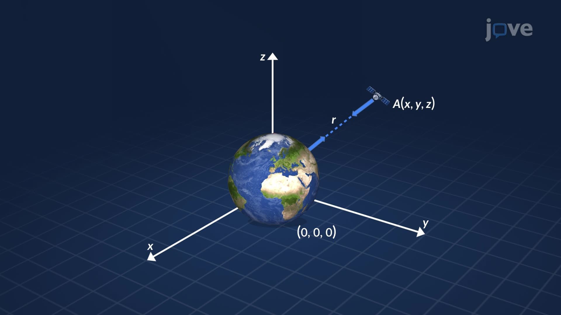
Before computing any integral, you need to define your vector field carefully. In atmospheric science, used operationally by agencies like NOAA and NASA's Goddard Space Flight Center, airflow is described by two quantities: a velocity vector field v (direction and speed of air) and a density scalar field ρ (how much mass per unit volume is present). Multiplying these together produces a new vector field F = ρv, often called the mass flux density. Every point on your surface now has an associated vector describing how much mass is trying to push through at that location.
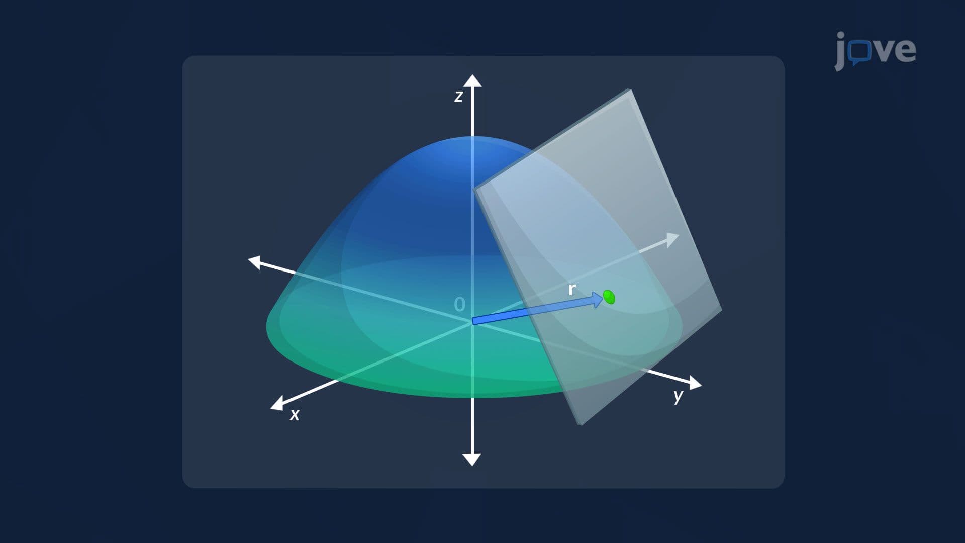
A surface integral of a vector field requires an oriented surface, one where you have consistently chosen which side is "outward" and which is "inward." This choice is captured by the unit normal vector n at every point. When F and n point in roughly the same direction, their dot product is positive, meaning flow is exiting the region. When they oppose each other, the dot product is negative, flow is entering. This sign convention is critical in real applications: in fluid mechanics and weather modeling, distinguishing inflow from outflow determines whether a storm system is intensifying or dissipating.
The integral itself is built the same way you learned Riemann sums in early calculus. Divide surface S into many small, nearly flat patches. On each patch: compute F · n (mass flow per unit area), then multiply by the patch's area ΔS. Sum all these products. As patch size shrinks toward zero and the number of patches grows without bound, this sum converges to the surface integral, the net flux of F across S. This limit process connects directly to ideas you encounter in AP Calculus BC and college-level Calculus III courses.
Flux in surface integrals doesn't stand alone. It links directly to several landmark theorems:
Together, these tools appear in college courses from Calculus III through differential equations and physics, and show up in engineering licensing exams, physics GREs, and advanced coursework at universities across the US.
Related Micro-courses