Loading subject page…


95 views


Video Summary: Extended Versions of Greens Theorem Explained
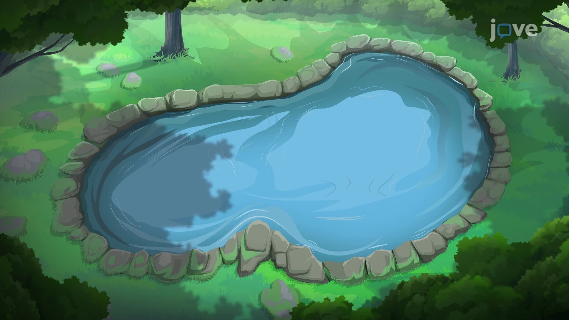
Can a single theorem handle regions with holes punched through them, like a lake sitting inside an island? Extended versions of Green's Theorem basics make this possible by cleverly extending the classic formula to complex, multiply-connected regions. Think of coastal engineering surveys along Florida's barrier islands, regions bounded by both outer shorelines and inner waterways. Watch the full video on JoVE Coach to master this concept with expert-led visuals and step-by-step explanations.
Green's Theorem is one of the most powerful tools in multivariable calculus. In its standard form, it equates a line integral around a simple closed curve to a double integral over the enclosed region. But what happens when that region isn't simple, when it has a hole in it, or when it's assembled from several pieces joined together? That's precisely where the extended versions of Green's Theorem come in, and understanding them is essential for any serious calculus student.
The classical statement of Green's Theorem assumes you're working with a simply connected region, one with no holes or interior voids. The boundary is a single closed curve, and the region lies entirely to the left as you traverse it counterclockwise. This works beautifully for shapes like circles, rectangles, or ellipses. But many real-world regions, a river delta cut through by channels, a metal plate with a circular hole drilled through it, or an annular region between two concentric circles, violate this assumption. Trying to apply the standard theorem naively to these shapes leads to incorrect results.
The key insight behind the extended versions of Green's Theorem is a technique called boundary decomposition. By introducing imaginary cuts, line segments that connect an outer boundary to an inner boundary, you split the holed region into two or more simply connected subregions. Each subregion now satisfies the conditions of the standard theorem. When you apply Green's Theorem to each piece and add the results, something elegant happens: the line integrals along the imaginary cut segments appear twice, once in each direction. Because they run in opposite directions, they cancel exactly. What remains are the integrals over the true physical boundaries, the outer curve and the inner curve, giving you the correct total.
This is not just a mathematical trick. It reflects a deep truth about how curl and divergence behave across regions, and it mirrors techniques used in Stokes' theorem and the divergence theorem, which generalize these ideas to three dimensions.
A critical detail that students often miss is boundary orientation. For the extended theorem to work correctly, positive orientation must be maintained throughout: the region must always lie to your left as you walk along the boundary. This means the outer boundary is traversed counterclockwise, while any inner boundary, surrounding a hole, is traversed clockwise. Reversing either of these flips the sign of the corresponding line integral, producing a wrong answer. This concept of consistent orientation carries directly into Stokes' theorem, making it a foundational habit to build early.
In AP Calculus BC and college-level multivariable calculus courses (Math 2400, Calc III), Green's Theorem problems frequently appear on midterms and finals. While AP Calculus BC does not test extended versions directly, understanding them builds the deeper intuition that shows up in free-response problems involving area calculation and flux. At the university level, extended Green's Theorem is a standard topic in courses that lead into real analysis and vector calculus. In applied settings, engineers at organizations like NASA or the US Army Corps of Engineers use these techniques when modeling fluid flow around solid obstacles, computing electromagnetic potentials in regions with excluded singularities, or analyzing stress distributions in holed structural components.
Related Micro-courses