Loading video…

 19 Concepts
 95 views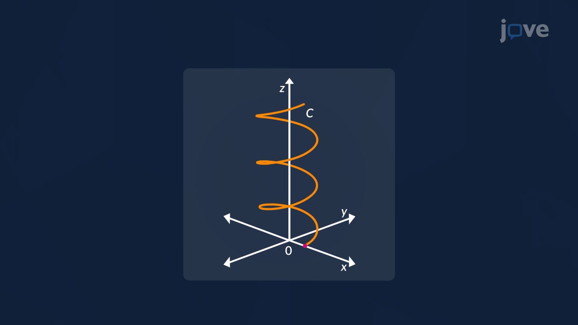

Video Summary: What are Line Integrals in Space
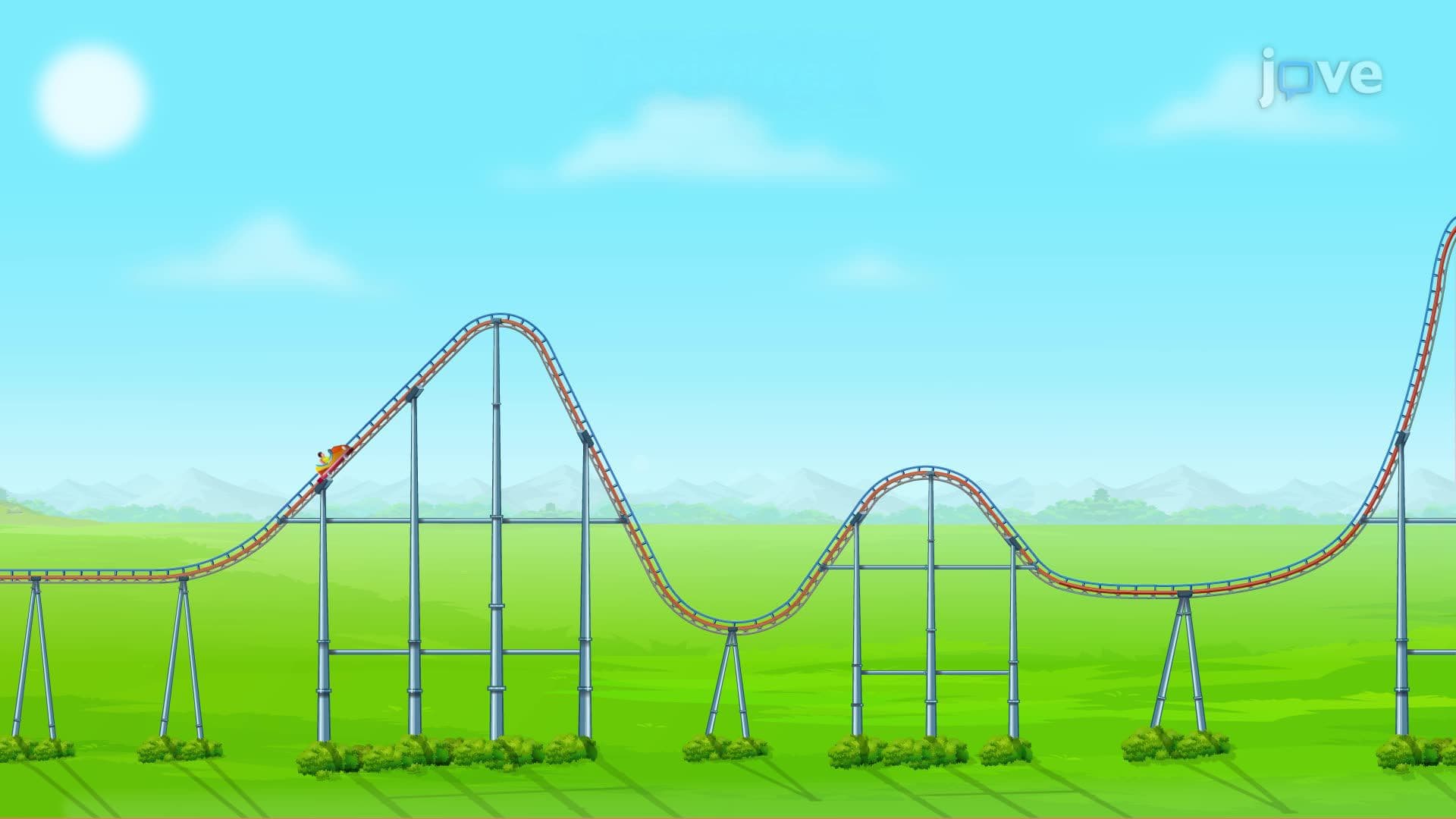
How do engineers calculate the total force on a roller coaster's curved track in three dimensions? That's exactly where line integrals in space come in. This concept extends integration along any 3D path, like a helical spring or NASA satellite orbit, by accumulating values point by point. Scalar versions handle quantities like mass; vector versions capture directional forces. Watch the full video on JoVE Coach to master this concept with expert-led visuals and step-by-step explanations.
A standard integral sums values along a straight number line. Line integrals in space push that idea into three dimensions, summing a function's values along any curved path, a helix, a spiral, a roller coaster loop, through 3D space. This makes them indispensable tools in multivariable calculus courses at US colleges and universities, and they appear frequently in AP Calculus BC extensions, university physics, and engineering curricula.
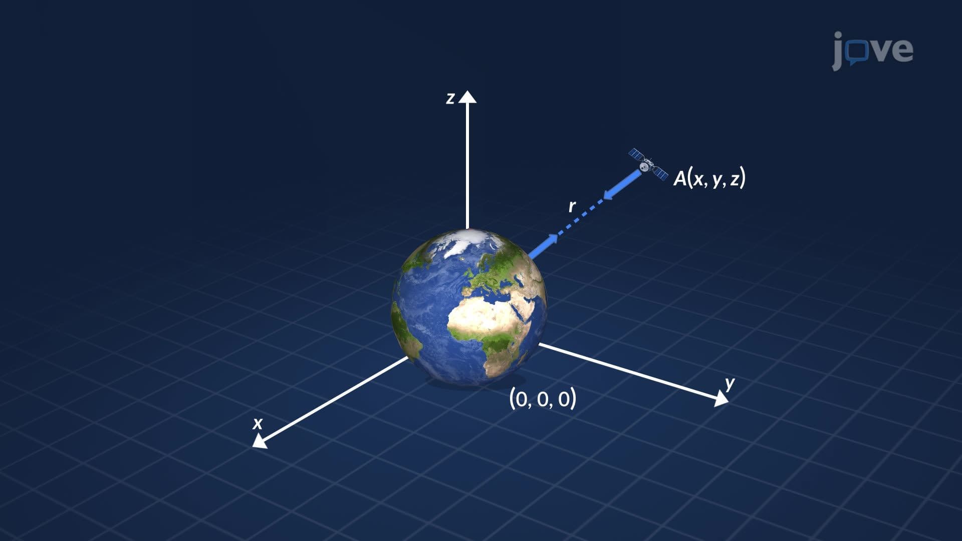
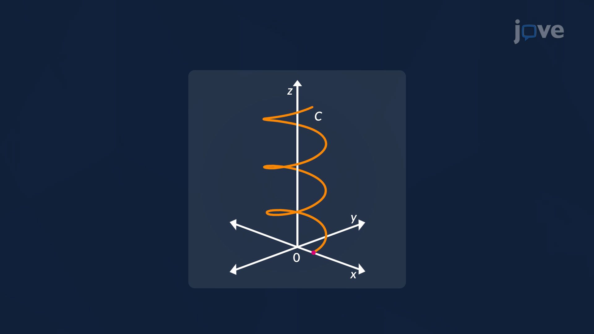
Every line integral in space begins with a parametric description of the path. A position vector r(t) = ⟨x(t), y(t), z(t)⟩ maps a single parameter, usually time t or an angle, to a point in 3D space. As t increases, r(t) traces a smooth, continuous curve called the trajectory C. For example, a helical spring can be described by r(t) = ⟨cos(t), sin(t), t⟩, where the x and y coordinates spin in a circle while z steadily rises. Mastering this parametric setup is the essential first step before evaluating any line integral.
When the quantity being measured has no direction, such as mass density, temperature, or electric charge, a scalar line integral is used. The function f(x, y, z) is integrated with respect to arc length ds, which naturally accounts for how quickly the curve moves through space. A classic US engineering problem involves finding the total mass of a thin wire or coiled spring when density varies along its length. The arc length element ds = |r'(t)| dt converts the problem into an ordinary single-variable integral, making computation straightforward once the parametrization is set.
When the path moves through a vector field F, such as gravity, electromagnetism, or fluid flow, a vector line integral measures the accumulated effect of the field along the curve. Only the component of F that points in the direction of motion (the tangential component) contributes to the integral. This is why the dot product F · dr appears in the formula: it filters out perpendicular forces that do no work. A concrete example is calculating the work done by gravity on a satellite following a curved orbit, or the work performed by an electric field on a charged particle moving through a cyclotron at a US national laboratory like Fermilab.
Line integrals in space are not isolated, they sit at the center of a powerful web of theorems. Green's theorem relates a line integral around a closed 2D curve to a double integral over the enclosed region. Stokes' theorem generalizes this to 3D surfaces, connecting a line integral around a boundary curve to a surface integral involving curl. The divergence theorem extends the logic further to volumes. Understanding conservative vector fields, where the line integral is path-independent, is equally critical. These connections appear on college midterms and final exams in Calculus III (Multivariable Calculus), a standard course at universities including MIT, UCLA, and state school systems across the US.
Related Micro-courses