Loading video…

 19 Concepts
 95 views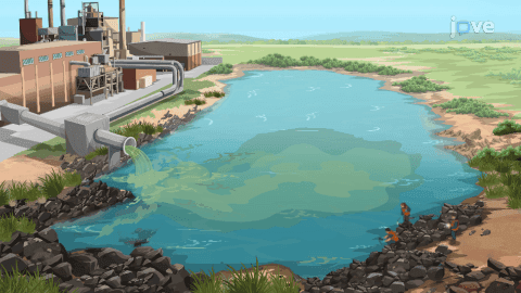

Video Summary: Vector Forms of Greens Theorem Explained
How do scientists track invisible pollutants swirling through a lake without walking every inch of its shoreline? The answer lies in understanding the vector forms of Green's Theorem. This powerful calculus concept connects boundary circulation to interior rotation in a vector field, eliminating the need for impractical edge-by-edge measurements. In a real US environmental monitoring scenario, scientists model pond water flow as a vector field, calculate its curl, and determine total pollutant circulation using just the pond's area. Watch the full video on JoVE Coach to master this concept with expert-led visuals and step-by-step explanations.
One of the most elegant results in vector calculus is Green's Theorem, which tells us something remarkable: instead of laboriously computing a line integral around a complicated closed curve, we can evaluate a double integral over the region it encloses, and get the exact same answer. The vector forms of Green's Theorem take this idea further by framing it in the language of curl and divergence, giving the theorem real physical meaning for students studying fluid dynamics, electromagnetism, and environmental science.
Green's Theorem has two primary vector interpretations: the circulation-curl form and the flux-divergence form.
The circulation-curl form states that the line integral of a vector field F around a positively oriented, simple closed curve C equals the double integral of the curl of F over the enclosed region D. In plain text:
∮(C) F · dr = ∬(D) (curl F) · k dA
Here, k is the unit vector pointing out of the plane, and (curl F) · k extracts the vertical component of the curl, the part responsible for in-plane rotation.
The flux-divergence form relates the outward flux of F across C to the double integral of the divergence of F over D:
∮(C) F · n ds = ∬(D) div(F) dA
This form answers a different question: instead of asking how much the field rotates, it asks how much the field spreads out or compresses within the region.
Understanding curl and divergence is essential to interpreting these vector forms. The curl of a vector field measures how much the field rotates around a point, think of a tiny paddle wheel placed in a stream. If the wheel spins, the curl is nonzero. The divergence measures whether the field is acting as a source (spreading outward) or a sink (converging inward) at each point.
In the pond-pollution scenario, the water velocity is modeled as a continuous vector field F. Calculating (curl F) · k gives a constant value, say, 2, meaning the water rotates uniformly across the entire pond. The total circulation around the shoreline then equals 2 × Area(D). No boundary traversal required. This same logic is applied by US environmental agencies like the EPA when modeling contaminant spread in lakes and river systems.
Green's Theorem is not an isolated result, it is a two-dimensional special case of Stokes' Theorem, which generalizes circulation-curl relationships to three-dimensional surfaces. Similarly, the flux-divergence form of Green's Theorem is a 2D version of the Divergence Theorem (also called Gauss's Theorem), which relates flux through a closed surface to divergence within the enclosed volume.
For students in college-level Calculus III or Multivariable Calculus courses at US universities, from community colleges to MIT OpenCourseWare users, mastering Green's Theorem is a gateway to understanding Maxwell's equations in electromagnetism and fluid continuity equations in engineering. On AP Calculus BC, while full Green's Theorem problems are not always tested, the foundational ideas of line integrals and area calculations appear regularly, making this concept highly valuable exam preparation.
When asked to apply Green's Theorem on a homework problem or college midterm, follow this structured approach:
1. Confirm eligibility, verify the curve C is simple, closed, and positively oriented (counterclockwise), and that F has continuous partial derivatives on D. 2. Choose the correct form, use the curl form for circulation problems, the divergence form for flux problems. 3. Compute the integrand, calculate (∂Q/∂x − ∂P/∂y) for the curl form, or (∂P/∂x + ∂Q/∂y) for the divergence form. 4. Set up and evaluate the double integral over region D using appropriate coordinate systems (Cartesian, polar, etc.). 5. Interpret the result, connect the numerical answer back to the physical or geometric context of the problem.
This structured method prevents the most common student errors: sign mistakes from incorrect orientation and misidentifying which partial derivatives to compute.
Related Micro-courses